# Chandler S. Reilly: full site text

---



---

Assistant professor of economics at Metropolitan State University of Denver.

---

Research in political economy and applied microeconomics.

---

# Can Markets Improve Recycling Performance?: A Cross-Country Regression Analysis and Case Studies

Elena C. Prenovitz, Peter K. Hazlett, Chandler S. Reilly (2023). Sustainability.
DOI: https://doi.org/10.3390/su15064785

## Abstract

Can recycling reduce negative externalities created by landfills? Environmentalists argue yes; however, the efficiency of recycling will be institutionally contingent. Entrepreneurs will face less barriers to profit from recycling in countries with more economic freedom. Additionally, recycling conducted by private firms will be more cost-effective and have higher rates of innovation in recycling technology relative to a nationalized industry. The purpose of this study is to test these claims. First, a two-way fixed effects regression model is estimated using panel data from 34 countries over the years 2000 to 2019. Our regression results show that increases in economic freedom have a positive effect on recycling rates, independent of related policy effects. Second, using two brief case studies of the Republic of Korea and Taiwan, we show how the inefficiencies of bureaucratic management suggest that private industry can be a less costly solution to encouraging recycling. The empirical results and case studies strongly suggest that increases in economic freedom can be an important mechanism for increasing recycling rates, and private industry involvement in existing recycling programs can limit unnecessary costs.

## 1. Introduction

For decades now, recycling has been among the popular "green habits" to adopt as part of daily life. Many cities require that residents separate their trash so plastic bottles, glass bottles, and paper products can all be sent off to be broken down and repurposed as raw material to be used in production. Recycling centers collect waste for a nominal fee. Companies loudly advertise their products are made from "100% recyclable materials". Common to many of these trends are policies intended to directly encourage recycling, whether it is through subsidies or the threat of fines when individuals do not comply. Missing from the popular and academic conversation surrounding recycling is how free markets may help or inhibit more recycling and increased recycling efficiency.

We argue individuals will find it in their self-interest to recycle, conditional on the institutions permitting such behavior. Recycling tends to be costly relative to the value it creates such that any additional costs (e.g., transaction costs) can inhibit the development of markets in recycling. However, more economic freedom can lower transaction and other costs, ultimately leading to a higher expected value in recycling. Economic freedom, as used here, refers to institutions such as strong property rights, limited government regulation, and freedom to trade. Higher levels of economic freedom, then, can promote higher levels of recycling relative to a situation where economic freedom is more restricted.

Many researchers have studied the relationship between institutions, such as democratic governance and economic freedom, and environmental issues. Clulow and Reiner [1], for example, examine how democracy affects energy transition, finding that democracy has a significant effect on low-carbon energy sources. Similarly, earlier work from Graddy [2] shows that increases in the level of democracy in a country can have significant positive effects on pollution reduction. Other research, more directly related to this paper, has assessed the relationship between economic freedom and environmental issues. Mahmood et al. [3] find evidence suggesting economic freedom can create an environment that encourages R&D activities that enhance energy-saving technologies and have a positive impact on the environment. Rapsikevicius et al. [4] present evidence from European countries showing mixed results of the effect economic freedom has on environmental performance and suggest a way to think about the optimal level of economic performance. Other tangentially related work has focused on the effect economic freedom can have on tourism [5]. Much of the research on the economics of recycling has focused on the efficiency of recycling and consumer behavior in recycling. For instance, Rapsikevicius et al. [6] propose a way of using blockchain technology in recycling programs to enhance coordination and efficiency in plastics recycling. Several other papers examine how entrepreneurship impacts innovation in recycling [7]; consumer perceptions of recycling [8]; consumer intentions to recycle at the end of a product's life using survey results and case studies [9,10]; and consumer recycling behavior in different settings [11,12]. These works, particularly those related to entrepreneurship, are conceptually linked to our focus on economic freedom. Countries with higher levels of economic freedom create the institutional conditions necessary to incentivize wealth-enhancing entrepreneurship [13]. However, existing research has not linked economic freedom to recycling specifically. Our intention is to bridge the gap between these two subjects by examining how institutions, specifically economic freedom, can affect recycling across countries using both panel data on 34 countries from 2000 to 2019 and two case studies.

The regression analysis using our panel data assesses the relationship between economic freedom and recycling rates while accounting for a variety of relevant controls and any year or country-specific heterogeneity to isolate our relationship of interest. Our regression estimates suggest there is a strong positive relationship between economic freedom and recycling rates, independent of policy effects. While those results do not illuminate the exact mechanism for this relationship, we explore how the strength of private industry and state intervention can affect recycling efficiency using two case studies. Not only do the case studies aid in understanding the mechanism by which economic freedom may positively affect recycling rates, they also complement the regression results in uncovering potential causal effects.

Our case studies examine recycling programs and industries in the Republic of Korea and Taiwan. These cases are useful for our purposes because they represent two examples where economic freedom moves in opposite directions, at least with respect to the management of recycling. In the Republic of Korea, the government implemented subsidies for recycling while leaving decision-making up to private industry for how to manage recycling. In Taiwan, the government nationalized the recycling industry. Both countries experienced increases in their recycling rates under drastically different policies. However, the institutional differences give reasons to believe that cost-efficiency across the two countries varies. the Republic of Korea's policies left recycling in the hands of private industry, allowing the incentives for cost minimization to guide decision making. In contrast, the nationalized recycling industry in Taiwan weakened the incentives for cost efficiency by leaving decision making up to government bureaucrats.

The empirical results and case studies presented in this paper contribute to the literature on free market environmentalism. Our evidence suggests that, despite the fact that our measure of economic freedom does not directly target recycling, it creates an environment conducive to more recycling by allowing individuals to exploit gains from trade. This also suggests that enhancing economic freedom along margins more directly related to recycling could have similar effects. The estimated relationship between economic freedom and recycling rates is also stronger than that between environmental policy stringency and recycling rates, suggesting further that economic freedom may play a more important role. If policymakers want to encourage more recycling, they can potentially make more progress toward this goal without resorting to costly subsidies, recycling requirements, or a nationalized industry.

The rest of the paper proceeds as follows. Section 2 lays out the economics of recycling and provides some theoretical justifications for why economic freedom can positively affect recycling. Section 3 presents our methodology including the data description and empirical strategy. Then, in Section 4, we present our regression results, estimating the relationship between economic freedom and recycling rates in OECD countries from 2000 to 2019. Additionally, Section 4 details changes in recycling policies in the Republic of Korea and Taiwan as case studies to better understand the relationship between economic freedom and recycling policy. Section 5 discusses our results and potential avenues for future research.

## 2. Theoretical Background

The generation, disposal, and treatment of waste are all issues faced by developed and developing countries alike. As countries become richer, people consume more, leading to more waste generation. This trend shows no signs of stopping in the future; as countries become more developed, more waste is projected to be created [14]. Something must be done with that waste, and much of it is commonly relegated to landfills. Landfills and incineration facilities have been found to generate a variety of negative externalities, such as air pollution, greenhouse gas emissions, and water contamination, among many others [15–25]. These concerns have led to efforts to encourage recycling and reduce the volume of waste making its way to landfills. Although recycling programs have been commonly implemented through various government policies, such as mandatory recycling or subsidies, recycling can also emerge through private incentives.

Suppose we have an individual who we will call Maren. Maren consumes some good until its use value eventually reaches USD 0[^1]. At that point, from Maren's perspective, the good turns into waste and will be disposed of. However, the fact that Maren now values the good at USD 0 does not imply there is no other individual who places a value above USD 0 on what is now considered waste. If there is another individual, we will call him Lee, who values Maren's waste at USD 5 because he can convert it into a usable material, then there is the possibility for gains from trade between Lee and Maren. Lee is willing to pay up to USD 5 for the waste and Maren is willing to accept any price above USD 0. Maren and Lee can exchange at some price between USD 0.01 and USD 5 and both parties will be made better off. The differences in valuations of what Maren considers waste lead to opportunities for trade, creating the incentives for individuals to recycle. In a zero transaction costs world, Maren would be able to sell any of her waste to someone such as Lee, who is willing to pay for it (attaches some positive value to her waste). However, in a world with positive transaction costs, the costs of exchanging may prevent these transactions from occurring, as the ability for Lee to profitably find and collect these items may be costlier than the profit he would make from using, or recycling, them. The higher a person such as Lee values the good, the more likely these trades will occur. However, the higher the transaction costs, the less likely these trades will occur. The magnitude of these transaction costs will be a function of the institutions under which these individuals exchange in. Under institutions with poorly defined property rights and significantly costly barriers to entrepreneurial action, transactions costs will be higher, leading to less transactions like the one between Maren and Lee. Countries with these institutions tend to be less economically free, as defined by the Economic Freedom Index [26], than countries with well-defined property rights and few barriers to entrepreneurial action. In contrast, more economically free countries will tend to have stronger property rights and lower transaction costs, making it more likely for private exchange in recycling to emerge, *ceteris paribus*.

[^1]: It is likely that Maren values the previously used good at some negative price, meaning she would be willing to pay someone to take the item. This item is then an economic bad, which is the opposite of an economic good. An economic good is something that individuals place a positive value on having a higher quantity. An economic bad, then, is something that individuals place a positive value on having a lower quantity. Waste is an economic bad. For simplicity, we assume the item's value is USD 0 in our example.

Even in a country with high economic freedom and significantly low transaction costs, there will always be some waste that cannot be profitably bought and used in a production process by an entrepreneur or consumed by someone with a positive consumer surplus. In such cases, negative externalities associated with waste disposal will still exist. Panel (a) in Figure 1 portrays this externality in the market for landfill services with a marginal social cost curve (*MSC*) having a higher price for a given quantity of landfill services relative to the marginal private cost curve (*MPC*). The societal optimal quantity of landfill services (*Q*) is less than the market equilibrium quantity (*Q<sub>e</sub>*). There are several possible remedies.

The first-best solution would be to better define property rights to internalize the externality, as recognized by Coase [27]. However, there are high transaction costs associated with defining property rights over the relevant margins to internalize the externality, such as the externalities methane emissions have on air quality and changing the environment. The next best solution would be to institute a Pigouvian Tax on landfill services to the point where marginal private cost equals marginal social cost, thereby leading to an equilibrium quantity of (*Q*)[^2]. As the price of landfill services increases with the tax, individuals will consume less landfill services. Although this leads to less waste being thrown into landfills, that waste may be placed in less desirable places through illegal waste-dumping activity. The unintended consequence to rising prices in landfill services is individuals engaging more in throwing their waste on public lands or even other people's property, as this type of disposal, although illegal, is a substitute for paying waste service fees[^3].

[^2]: Numerous studies have analyzed the effects taxes have on waste [28–30]. For a discussion and economic analysis of the optimal waste tax, see Kinnaman [31].

[^3]: Multiple studies find that increasing waste taxes lead to increased illegal waste dumping [32–39]. Perhaps the most thorough investigation of illegal waste dumping, or "fly-tipping" as it is called in England, is Liu et al. [37].

An alternative solution to a tax, and a common policy in many countries, is to subsidize recycling services. Recycling is a substitute for landfill services. A subsidy lowers the relative price of recycling to landfill services, leading to more waste being recycled and less thrown into landfills[^4]. The effect a recycling subsidy has on the market for landfills is shown in Panel (b) of Figure 1. The demand, or marginal benefit, for landfill services falls because the price of recycling has fallen with the subsidy. The new equilibrium is at *E′*[^5]. Even though there still exists dead-weight loss in this market because *MPC ≠ MSC*, the quantity is the same as that reached at equilibrium *E\**, the intersection of *MB* and *MSC*. Through the subsidy for recycling, the original optimal quantity of landfill services in the market without the subsidy is reached[^6]. There are multiple ways a government could subsidize recycling services. On one end of the spectrum, the government could pay private market actors the subsidy for recycling a certain quantity of waste. Alternatively, on the other end of the spectrum, the government could create a nationalized recycling industry where all recycling services are conducted by the state[^7]. The efficiency of recycling will depend upon which end the policy falls.

[^4]: For recent studies comparing waste taxation and recycling subsidy regimes, see Helm et al. [40] and Hua et al. [41].

[^5]: Although the socially optimal quantity from the original graph in Panel (a) is reached, this is not the new socially optimal quantity with the subsidy included.

[^6]: For a similar analysis on the economics of recycling subsidies, see [42] (pp. 486–487).

[^7]: Policies could fall between these two ends. For instance, government services may collect recycling waste and transport it to private recycling producers who they contract with. Or, some items could be recycled in the market while others relegated to government recycling facilities.

**Figure 1: The market for landfill services.** *Figure available in the published version.*

There are three main reasons why we might expect a private recycling industry to be more efficient than a nationalized industry. First, private firms will have stronger incentives to reduce the cost of their services relative to bureaus. Second, private entrepreneurs will have more incentive to innovate recycling technology that will make the recycling process more efficient. Finally, the government faces a knowledge problem when trying to centrally plan the recycling industry. Private entrepreneurs and bureaucrats operate in different institutions under different incentive structures[^8]. Firms seek to maximize profit by producing the most demanded goods and services at the lowest cost. Thus, firms will actively seek to minimize the cost of production to reap larger profits. Since bureaucrats do not internalize the cost of producing their output, cost minimization incentives are weaker. For the bureaucrat, reducing costs will not increase net benefits unless budget increases are tied to cost effectiveness.

[^8]: See Hazlett and Reilly [43] for a discussion of how entrepreneurial action differs in the marketplace and bureaucracy.

When it comes to the production process, private firms stand to gain large profits if they can improve the efficiency of their production processes through innovation. Alternatively, the bureaucrats face disincentives for increasing the efficiency of their production processes. If a bureau produces the same output with less resources than before, it is in their political sponsors', the politicians who directly support the bureau, interests to allocate less budgetary funds to that bureau. As far as bureaucrats are interested in maintaining their job and salaries, they will seek to avoid such action[^9].

[^9]: Bureaus have often been modeled as budget maximizing agencies [44]. If this is the case, then bureaus may face incentives to be less efficient in their production process as a strategy to increase their budgets.

Even if the government is able to overcome the hurdles of bureaucracy outlined above, they still face a knowledge problem with having to allocate resources in the nationalized industry. They would have to know the best location for recycling centers and the optimal size of each facility. Since not all waste is the same and some is easier to recycle than others, the government must decide which types of waste should be recycled. Finally, central planners would need to be able to effectively evaluate and innovate the recycling process. In a market for recycling services, this knowledge comes to fruition through the competitive market process. Firms in the wrong location, too small to take advantage of economies of scale, or too big to handle diseconomies of scale, will shut down. When waste cannot be profitability recycled, it will not be recycled at all. Entrepreneurs alert to profit opportunities will incessantly be searching for profitable recycling opportunities. Those who adopt the most cost-effective production techniques and technology will succeed, while those failing to do so will exit the market. Ultimately, there are mechanisms built into the market process to find solutions to these problems, which will prove increasingly difficult for central planners to solve.

We have discussed three main reasons why free markets and private industry may lead to better recycling outcomes than a regulated or nationalized industry in recycling. Exchanges which could divert waste from landfills are more likely to happen in more economically free countries with less barriers to entrepreneurial action and voluntary exchange. Even if the desired level of recycling is not brought about through private recycling efforts, a subsidizing private industry is likely to have better recycling outcomes because private actors will seek to lower the production costs of recycling and will constantly seek more efficient recycling methods[^10]. Additionally, when recycling is the responsibility of a government agency, there will be greater opportunities for mission creep and the growth of the bureau in other areas. Knowledge problems will be mitigated in the market through competition and profit and loss signals.

[^10]: The production costs of recycling do not only have economic effects, but also environmental effects. The fewer resources and energy used to recycle, the lower the carbon footprint of the recycling process, see Soltanian et al. [14] for a discussion of some of these effects.

## 3. Methodology

### 3.1. Data Description

The variables for our econometric analysis are collected from the Fraser Institute [45] and the OECD Stat database [46]. Brief descriptions and sources for all variables can be found in Table 1. What follows is a more detailed description of the data set.

**Table 1.** Variables and data sources.

| Variable | Source | Definition |
|---|---|---|
| Economic Freedom of the World Index | Gwartney et al. [45] | Index value ranging from 0 to 10, measuring the level of economic freedom in a country-year. |
| Recycling Rate | OECD [46] | Percentage, from 0 to 100, of waste diverted from waste streams for recycling (i.e., reprocessing of material) in a given country-year. |
| Material Footprint Per Capita | OECD [47] | Volume of raw material extracted to meet the final demand of an economy in thousands of kilograms in a given country-year. |
| Environmental Taxes | OECD [48] | Tax revenue generated by environmental policies as a percentage of total tax revenue in a given country-year. |
| Environmental Policy Stringency Index | OECD [49] | Level of environmental policy stringency, ranging from 0 to 6, in a given country-year. |
| GDP Per Head | OECD [50] | GDP per head in 2015 USD constant prices and constant PPP in a given country-year. |

We collect data on a panel of 33 OECD countries and Brazil from 2000 to 2019[^11]. The empirical analysis in this paper is limited to OECD countries due to data availability issues. While the Economic Freedom of the World (see full description below) has data on many more countries, other variables including those on recycling rates and environmental policy used below are only available for OECD countries. Our results, then, should be interpreted with some caution, as we do not claim the results are applicable outside of our sample (e.g., countries on the continent of Africa). The full data set is unbalanced, with some countries having as few as one year of data for all variables. Our analysis uses both the unbalanced panel and the balanced panel after dropping any country that does not have data in every year from 2000 to 2019. The balanced panel contains 16 OECD countries from 2000 to 2019. The list of countries in our data set and the number of years they appear are reported in Table 2. Below is a description of the variables we use in our regression analysis.

[^11]: Ideally, we would have complete data on all OECD countries. Colombia, Costa Rica, Latvia, Lithuania, and New Zealand do not have complete data available across our sources and are omitted.

**Table 2.** Countries and number of years available in full panel from 2000 to 2019.

| Country | Years | Country | Years |
|---|---|---|---|
| Australia | 14 | Italy | 20 |
| Austria | 20 | Japan | 20 |
| Belgium | 20 | Korea, Rep. | 13 |
| Brazil | 1 | Luxembourg | 13 |
| Canada | 8 | Mexico | 11 |
| Chile | 5 | Netherlands | 20 |
| Czech Republic | 20 | Norway | 19 |
| Denmark | 20 | Poland | 20 |
| Estonia | 6 | Portugal | 16 |
| Finland | 20 | Slovak Republic | 14 |
| France | 20 | Slovenia | 11 |
| Germany | 20 | Spain | 20 |
| Greece | 12 | Sweden | 20 |
| Hungary | 20 | Switzerland | 20 |
| Iceland | 2 | Turkey | 4 |
| Ireland | 16 | United Kingdom | 20 |
| Israel | 6 | United States | 19 |

To analyze the relationship between economic freedom and recycling rates, we use the Economic Freedom of the World Index constructed by the Fraser Institute [45]. The index is internationally comparable and captures economic freedom based on five key areas that are summarized in the index value appearing in our regressions. The five areas include the size of government, legal system and property rights, sound money, freedom to trade internationally, and regulation [26]. Each of these five areas has several sub-components that are inputs to the summary index value. Yearly summary index values are restricted to the years from 2000 to 2019 to match the data from the OECD stat. The summary index ranges in value from 0 to 10, where 0 represents the lowest level of economic freedom and 10 represents the highest level of economic freedom. We restrict the countries from this data set to those matched with the OECD data described below.

The dependent variable in our regressions is the recycling rate collected from the OECD stat [46]. This variable measures the percentage of waste that is diverted from waste streams for recycling. Waste as captured in this measure includes household and similar waste, such as that generated by small businesses, office buildings, and institutions. Recycling is defined in the OECD database as follows:

> any reprocessing of material in a production process that diverts it from the waste stream, except reuse as fuel. Both reprocessing as the same type of product and for different purposes are included. Direct recycling within industrial plants at the place of generation is excluded.

The control variables in our regressions are also collected from the OECD stat database. The first is GDP per head in 2015 USD constant prices and constant PPP [50]. Our intention with this control is to hold constant any wealth effects that may influence the recycling rate within countries over time. Although it is likely that including the GDP measure quadratically is most appropriate to capture any Kuznets-type relationship, we are unable to do so given our dataset. The matrices to estimate our regression coefficients are not invertible when squared GDP is included, we are limited to including GDP per head alone. The data on GDP ranges from USD 11,000 per head (Brazil) to over USD 114,000 per head (Luxembourg) and has a standard deviation over USD 15,000.

We have data on the material footprint per capita, which measures the volume of raw material (in thousands of kilograms) extracted to meet the final demand of an economy [47]. This measure may have a relationship with the production of waste and treatment through recycling not captured by our other control variables. Recycled materials and raw materials are to some degree substitutes in production. As a country recycles more, we would expect that raw material extraction will decline, holding all else constant.

Our final two variables are related to environmental policy and are included to capture policy effects that may be related to both economic freedom and recycling rates. The first is environmental tax revenue as a percentage of total tax revenue [48]. In our sample, this variable ranges from 12.1 to 13.8, suggesting that in some countries environmental subsidies exceed environmental taxes on net. The second is the Environmental Policy Stringency (EPS) Index [49]. This is a country-specific and internationally comparable measure of environmental policy stringency bounded between 0 and 6, where 6 represents the highest level of stringency and 0 represents the lowest level of stringency. The average value of this index in our data is 2.7 though there is considerable variation across and within countries. For example, between 2000 and 2018, the EPS Index in the United States rose from 1.2 to 2.9, suggesting that environmental policy became substantially more stringent over this period.

Although the environmental taxes and the environmental policy stringency variables are related to environmental policy in general, we expect that these variables will have some relationship with recycling rates. Environmental policies may include taxes on waste or subsidies for recycling, both of which are likely to induce higher recycling rates, but the expected direction of the relationship between our environmental tax revenue variable and recycling rates is ambiguous. Increases in recycling subsidies will reduce this measure of environmental tax revenue, while increases in taxes on waste will increase it. Both changes may lead to increases in recycling rates. Regardless of the direction of the effects, including the measure of the environmental tax revenue and the EPS Index will aid in disentangling the effects of economic freedom directly and any potential induced policy response related to economic freedom [2]. Summary statistics for all our variables can be found in Table 3.

**Table 3.** Summary statistics.

| Variable | N | Mean | St. Dev. | Min | Max |
|---|---|---|---|---|---|
| EFW Index | 510 | 7.772 | 0.429 | 5.800 | 8.850 |
| Recycling Rate | 510 | 23.427 | 11.685 | 0.106 | 59.929 |
| Material Footprint Per Capita | 510 | 27.291 | 11.437 | 10.154 | 88.703 |
| Environmental Taxes | 510 | 6.863 | 2.391 | 12.140 | 13.810 |
| Environmental Policy Stringency Index | 510 | 2.706 | 0.841 | 0.000 | 4.722 |
| GDP Per Head (thousands) | 510 | 42.058 | 15.548 | 11.421 | 114.805 |

Figure 2 shows a scatter plot of economic freedom values and recycling rates in a given country-year for our entire data set and the simple linear relationship between the two variables estimated using Ordinary Least Squares (OLS). There is a strong positive relationship, suggesting that more economic freedom may have a positive impact on recycling rates. However, this relationship may be due to other factors correlated with economic freedom, recycling rates, or both. We address this issue using the empirical strategy described in the following section.

**Figure 2: Economic freedom of the world index and recycling rates.** *Figure available in the published version.*

### 3.2. Empirical Strategy

Our strategy to obtain a better estimate of the relationship between economic freedom and recycling rates is to control for relevant factors, such as GDP and policy variables, and introduce time and country-specific fixed effects. In doing so, we can quantify the relationship between economic freedom and recycling rates independent of those relevant controls and any unobserved heterogeneity specific to a given year or country. The econometric model based on this strategy is given by the following equation:

*Y<sub>i,t</sub>* = *b<sub>1</sub>EFW<sub>i,t</sub>* + **X**<sub>*i,t*</sub>**G** + *a<sub>i</sub>* + *a<sub>t</sub>* + *e<sub>i,t</sub>*. (1)

*Y<sub>i,t</sub>* is our outcome variable of interest, recycling rates which are bounded between 0 and 100. Recycling rates are bounded in this way because, in the extremes, either no waste is diverted to recycling or all waste is diverted to recycling given the definition of recycling rates. *EFW<sub>i,t</sub>* is economic freedom for country *i* in year *t*, and *b<sub>1</sub>* is our coefficient of interest. **X**<sub>*i,t*</sub> represents a matrix of our control variables including GDP per capita, material footprint per capita, environmental tax revenue as a percentage of total tax revenue, and the environmental policy stringency index. **G** is a vector of regression coefficients for the control variables. Country and year fixed effects are given by *a<sub>i</sub>* and *a<sub>t</sub>*, respectively. Errors are given by *e<sub>i,t</sub>*.

We estimate this model using the full unbalanced panel of data and the balanced panel of data using a within-panel estimator and the "plm" package in the statistical software R. Standard errors are clustered at the country level and heteroskedasticity robust. The purpose of the two-way fixed effect approach here is to control for any unobservable characteristics that may be unique to a specific year or specific country as a way to isolate the relationship between economic freedom and recycling.

We test for misspecification using a Hausman test to ensure that the fixed effects model is appropriate in contrast to random effects using our base regression model with both country and year fixed effects against a model with the same controls and random effects instead of the original fixed effects. The null hypothesis of the Hausman test is that country specific errors are correlated with regressors. Failing to reject the null hypothesis would suggest that a random effects model is preferable to a fixed effects model. The results of this test strongly reject the null hypothesis, suggesting that our fixed effects specification is appropriate for this context.

We also face the choice of whether to include year fixed effects. Two tests used to confirm year fixed effects are necessary. First is a Breusch–Pagan test, which is a Lagrange multiplier test on a model including county fixed effects alone, where the null hypothesis is that there are no significant time effects. Second is a simple partial F-test of models with and without year fixed effects where the null hypothesis is that there is no joint effect of year fixed effects. Failing to reject the null hypothesis in either of these tests would suggest that the year fixed effect may not be necessary. However, the results of both tests for the unbalanced and balanced panels suggest year fixed effects are necessary as the null hypotheses are strongly rejected. Therefore, our preferred specification is the two-way fixed effects regression with our set of controls that will estimate the effect of changes in economic freedom on recycling rates within the countries in our sample. The results for each of the specification tests are reported in Table 4 using both the unbalanced and balanced panels of data.

**Table 4.** Specification tests.

| | (1) Hausman Test | (2) Breusch-Pagan Test | (3) Partial F-Test |
|---|---|---|---|
| Unbalanced Panel | 50.69 *** | 6.83 *** | 3.32 *** |
| Balanced Panel | 73.98 *** | 5.83 ** | 2.64 *** |

Note: \*\* *p* < 0.05; \*\*\* *p* < 0.01.

## 4. Findings

### 4.1. Regression Results

Our regression estimates using both unbalanced and balanced panels are reported in Table 5 where the control variables are those as described in Section 3.1 and both country and year fixed effects are included in both regressions. The first column of Table 5 shows the results for the unbalanced panel. In this estimation, economic freedom has a large and statistically significant effect on recycling rates. The standard deviation of economic freedom in the unbalanced panel is around 0.8, and our estimates suggest that a one standard deviation increase in economic freedom results in a nearly nine percentage point increase in recycling rates. This effect is equivalent to a 0.75 standard deviation increase in recycling rates. Compare this to the effect that an increase in environmental tax revenue has on recycling rates. A one standard deviation increase in environmental tax revenue (2.4 percentage points of total tax revenue) increases recycling rates by only 0.12 standard deviations. These results suggest that increases in economic freedom can have large effects on recycling rates independent of direct environmental policy effects. This is not to say that policies targeting recycling are unimportant. Rather, increases in economic freedom can create the conditions that make it in people's interest to recycle more. Although the exact mechanism(s) cannot be determined by our results, it is likely that increases in economic freedom through changes such as stronger property rights give people the ability to capture the value of turning waste into recycled materials. A further limitation of these results is that we cannot be sure we are estimating a causal effect. The fixed effects and controls do help isolate the effect of economic freedom on recycling rates, but there are likely other omitted variables that prohibit us from properly identifying the causal effect. For example, we do not have data on a recycling-specific environmental policy that would be associated with recycling rates and be possible with economic freedom. The omission of such a variable introduces the potential of bias in our estimates. While we are confident that the included fix effects help to address this issue, a causal interpretation of our estimates should be avoided.

**Table 5.** The effect of economic freedom on recycling rates.

Dependent Variable: Recycling Rate

| | (1) Unbalanced Panel Results | (2) Balanced Panel Results |
|---|---|---|
| EFW Index | 10.996 *** (1.431) | 13.745 *** (1.891) |
| GDP Per Head (thousands) | 0.054 (0.083) | 0.161 (0.185) |
| Material Footprint Per Capita | 0.020 (0.046) | 0.043 (0.105) |
| Environmental Tax Revenue | 0.604 *** (0.160) | 1.672 *** (0.343) |
| Environmental Policy Stringency | 0.667 (0.616) | 0.022 (0.704) |
| Observations | 510 | 320 |
| R<sup>2</sup> | 0.170 | 0.258 |

Note: \*\*\* *p* < 0.01.

Similar results hold for the estimates using the balanced panel reported in the second column of Table 5. The section that follows will discuss two case studies to further touch on potential mechanisms and causal evidence for the results found here by focusing on the interactions between recycling policies and outcomes associated with economic freedom.

### 4.2. Case Studies

In recent years, the Republic of Korea and Taiwan have become two of the only non-European countries to enter the ranks of the world's top recyclers. As East Asian countries, the Republic of Korea and Taiwan have had different development paths from their European counterparts, making them interesting cases to examine recycling under different policy regimes. While both countries rely on subsidies to spur recycling, the Republic of Korea utilizes a private market for recycling industry while Taiwan has transitioned from private recycling to nationalized recycling centers.

#### 4.2.1. The Republic of Korea

In 2018, the Republic of Korea became the only non-European country to rank in the top-five leading recyclers in the world [51], and had the highest recycling rate of the year, 61.57% [46]. This is a new trend for the nation, with their recycling rate more than doubling since 1994 [52]. The Republic of Korea's unique waste management system may shed light on this phenomenon.

The Republic of Korea's modern waste management system is neither completely public nor private and developed very rapidly after a series of major policy changes beginning in the late 1980s. The defining feature of these policy changes was a change in the assignment of property rights over recycling management. From the end of the Korean War to the early 1990s, waste in the Republic of Korea was managed under a public regime [53]. During this period, the cost of waste management was negligible to both households and firms. Because the Korean War virtually decimated all industry in the Republic of Korea, very little waste was generated in the Republic of Korea in the early years of its existence [53]. However, industry in the Republic of Korea rapidly developed and large-scale waste was being produced by the late 1970s. Until 1993, all waste created from the entirety of the Seoul metropolitan area and surrounding rural areas was collected by the municipal governments and dumped in the Nanji landfill [52,53].

In the late 1980s, the Korean government began to notice that the Nanji landfill would soon reach capacity [52,53]. Not only was the site running out of space for dumping, but Seoul citizens were beginning to raise health concerns regarding the pollution resulting from the decaying mountain of garbage and waste incineration [52–54]. The government initially proposed building a multitude of new landfill sites around Seoul; however, these plans received severe public backlash. Similar to NIMBY attitudes towards multi-family housing, many residents of Seoul and surrounding areas strongly opposed the construction of a landfill near their community. The federal government responded by passing the Waste Control Act of 1986. The aim of the Waste Control Act was to reset the framework for waste management and prepare the Republic of Korea for the policy changes that would follow it [52,53,55,56].

The Republic of Korea uses a hierarchical structure for its waste management policy agenda. Before the Waste Control Act, incineration and landfill were at the top of the policy hierarchy, followed by waste reduction and utilization [52,53,55]. The Waste Control Act flipped the policy agenda such that reduction and utilization were at the top and landfill and incineration were pushed to the bottom. This shift allowed for a stream of policies to be passed over the course of the following decade with the intent of reducing municipal waste and rebuilding the waste management system. Of these policies, three made the most significant difference in waste management practices. Two of these policies were targeted towards producer waste and one policy was targeted towards household waste. The first of the producer-focused policies, the Deposit Refund System (DRS) enacted in 1993, was aimed at spurring recycling practices in producers of designated recyclable outputs. Second, the Extended Producer Responsibility (EPR) system of 2003 replaced the DRS. In order to address household waste, the implementation of the Volume-based Waste Fee (VWF) system in 1995 made households bear the cost of their waste for the first time [52–55].

The DRS and EPR policies targeted producer responsibility over waste. The DRS policy created a system in which producers of designated outputs were given the option to either pay the municipal government a fee to dispose of their waste via landfill or incineration, or they could recycle their waste and receive a refund for the disposal cost [52,53,55]. This fee was referred to as the "deposit rate" and was a rate of Won per kilogram set by policymakers that varied by industry. The deposit rate was the price at which producers would pay to have their waste deposited in a landfill by the government, or on the flip-side, what producers would be refunded if they recycled their waste. Effectively, the government was attempting to make producers bear more of the cost of their waste while simultaneously subsidizing recycling.

Prior to the enactment of DRS, Korea lacked recycling infrastructure and there was no private industry for recycling. At the time of implementation, many firms in industries where recycling costs of their products were relatively low, such as tires, glass, lubricants, and batteries, quickly developed recycling infrastructure to reap the benefits of the refund. Shortly after the implementation of DRS, demand for both private recycling facilities and recycled products grew, resulting in a quickly developing private recycling industry. Several producers even built recycling facilities that offered nation-wide recycling services.

Some industries opposed DRS in its early years. These industries mainly consisted of producers of durable goods, such as home appliances, and other products that were very costly to recycle. They argued that the lack of recycling infrastructure made it impossible to recycle their waste and they were unable to receive the refund other industries benefited from. As the recycling sector developed, some of these industries that initially resisted DRS began to invest in recycling innovation and partake in recycling to receive the refunds. Over the course of the DRS era, the ratio of refund to deposits steadily increased. The refund-to-deposit ratio was two percent in its first year, but reached fifty-two percent after a decade [53] (p. 4).

The EPR system had the same goal as the DRS: make producers responsible for their waste. The methods of achieving this goal, however, were very different. Under the new system, the government discarded the refund mechanism to incentivize producers to recycle and instead requires producers to recycle a specific percentage of their waste each year. The required rate of recycling is gradually increased over time. The EPR system is still in place today and regulates the production of 24 products [53] (p. 7). The EPR system faced virtually no resistance from the affected industries. By the time of the implementation of EPR, there was a robust private sector for recycling and recycled products in the Republic of Korea, as mentioned before. The development of this sector, thanks to DRS, made the transition to EPR very smooth. Because a certain rate of recycling is required under EPR, all regulated industries meet this requirement and the program is viewed as a success. Due to this command-and-control program, the industries that were recycling at very low levels under DRS were forced to reach the new recycling requirements; however, there has been no change in behavior of firms that began recycling in the 1990s.

#### 4.2.2. Taiwan

Similar to the Republic of Korea, Taiwan emerged as an East Asian leader in recycling in recent years. Since 2019, Taiwan has maintained a recycling rate of about 56%, the world's second highest behind Germany. While they both climbed the ranks of "sustainable" countries in the past few decades, the Republic of Korea and Taiwan have had fairly different policy approaches to waste management. Taiwan provides a case where a once fully private market for recycling was crowded out by a central authority.

Beginning in 1989, the federal government of Taiwan began a four-stage system to move recycling in the country from the private market to a more nationalized industry [57,58]. The aim of the four-stage system was to slowly transition recycling from private to public over time as the EPA, a budget-maximizing bureau, exhibited mission creep.

The first stage, which lasted from 1989 to 1994, primarily involved identifying 17 items that would be regulated to be recycled and determining and implementing these regulations. These regulations were suggested by special committees whose members consisted of leaders in the industries of the regulated items. In addition, the Taiwan EPA set annual mandated recycling rates for each regulated item and monitored the relevant industries.

Stage 2 of the program lasted from 1994 to 1996. During this phase, the government began to increase involvement in the recycling industry. During Stage 1, the government faced many issues with monitoring the recycling industry, such as lack of transparency and false data reporting. To solve these issues, they established the Reduction, Recycling, and Reuse Foundation (3R Foundation), a non-profit government organization [57]. The aim of the 3R Foundation was to obtain contracts with the regulated industries that would give them the rights to take over recycling their products. They were successful on this front with the vehicle industry and handled recycling abandoned vehicles through their own shredding plant. However, 3R was unsuccessful at obtaining contracts with other industries.

Stage 3 was very short but very significant. From 1997–1998, Taiwan's Environmental Protection Administration (EPA) overhauled the entire recycling industry by establishing eight "recycling fund" committees to manage the entire industry. The committee members were selected by the EPA, their funds were public, and their budgets required EPA approval. Initially, the committees were overseen by the EPA but operated independently, similarly to a central bank.

In Stage 4 of the system, which was implemented in 1998 and persists today, the committees were fully centralized under the EPA. From the changes made during Stage 4, 28 items faced mandatory recycling programs and were required to pay fees for this recycling to the Resource Recycling Fund Management Committee, a new layer of bureaucracy that was responsible for overseeing and managing the eight recycling fund committees. The Resource Recycling Fund Management Committee is then overseen by parliament.

These changes have resulted in a highly regulated system for recycling. Producers and importers of regulated items are required to register with the EPA and must pay a fee and have their items recycled at their end-of-life. The funds from the fees paid are collected and managed by the recycling fund committees. Most of the funds are allocated towards subsidies to the industries that are mandated to recycle; however, the EPA is able to use these funds for essentially anything they deem fit.

The four-stage system was highly effective in propelling Taiwan to a top recycling rate, and Taiwan's EPA is continuously praised for policy success. However, there are a number of studies showing the achievement of this recycling rate is accompanied by a myriad of flaws. Some studies have questioned the efficiency of the state-sponsored recycling operations. Chen et al. [59] (p. 1667) assess the effects of the policy regime in the end-of-life vehicle recycling market. Prior to the policy change, there was a robust private market for the secondary recycled parts of vehicles, such as batteries and engine parts, as these scraps are valuable resources. The authors find that the nationalized recycling operators lack sufficient focus on auto shredding residue pollution, it is unclear whether the recycling fee will stimulate green innovation from producers, the Recycling Fund Management Committee shuts down illegal recycling operations that account for a significant amount of end-of-life vehicle recycling, and many of the recycling operations have very high energy costs that are not considered when assessing their environmental impact. Hsu and Kuo [60] note that recycling operators of home appliances are almost entirely supported by federal funds, and it is highly questionable whether these operations are cost-effective. Shih [61] discusses two weakness of the policy regime in the context of E-waste recycling: the policy eliminates competition between recyclers, and the imposed recycling standards have very high monitoring costs. Similarly, Chang [62] argues that some policy changes need to occur to promote more competition in the recycling of scrap tires. Wen et al. [63] question the ability of EPA performance indicators to accurately assess recycling performance.

While this handful of studies assesses industry-specific problems, there is clearly a pattern in the recycling regime. A high recycling rate achieved through nationalization seems to come at the cost of competition between recycling operators, lags in technological innovation, increased monitoring, and unclear performance assessments, all typical benefits of the private market. The root of these issues with the current regime stems from the fact that the Taiwan EPA faces the planners problem. The Recycling Fund Management Committees do not have complete knowledge in order to efficiently allocate funds, calculate the optimal recycling rate, organize operators, etc. One overarching issue with the efficiency of the regime identified by Ye et al. [64] is the number and location of recycling centers. Ye et al. [64] suggest that there are currently too many recycling centers and that these centers are too far from many collection depots. It might be more efficient to reduce the number of centers and relocate them closer to collection depots. If the profit–loss mechanism was more prevalent for recycling operators, these types of issues would be mitigated much more efficiently. Similarly, Lee and Na [65] note that the majority of recycling in Korea is performed by small- to medium-sized private operators, whereas in Taiwan the only legitimate operators are the large state-sponsored centers. Because of this, producers in the Republic of Korea provide more support, communication, and information to recycling operators, whereas in Taiwan the producers are relatively disconnected from the recycling centers. Tsai et al. [66] also discuss some regulatory issues of the system, such as vague regulatory definitions. It is impossible for the EPA and subsequent Recycling Fund Management Committees to evade these issues as the government mechanism necessarily faces a knowledge problem. Overall, it is unclear whether the benefits from reaching the 56% recycling rate outweigh these costs.

## 5. Discussion

Can markets improve recycling performance? If transaction costs are high from economically restrictive state regimes, then recycling is less likely to occur. Alternatively, under more economically free institutions, entrepreneurs will be more able to seize profit opportunities from converting waste to economic goods. This is supported by the findings of this study. The regression results in Section 4.1 showed a relationship between economically free countries and higher recycling rates. Although we cannot be certain of the exact mechanism causing the correlation from our empirical findings, the case studies of countries who relied more on private industry, a prominent organizational feature of economically free countries, tend to have more efficient recycling processes. These results suggest that if countries are concerned with increasing their recycling rates and the efficiency of their recycling industry, they can do so by increasing economic freedom. Economically free institutions allow entrepreneurs to profit more from converting waste to something of value.

This paper bridges the gap between the literature on the relationship between institution and environmental problems and on the economics of recycling. We show how institutions that promote entrepreneurship through economic liberalism can increase recycling rates and efficiency. However, even in the most economically free country, the private recycling market may not be able to lower the negative externalities associated with landfills to desirable levels. In this situation, subsidizing private recycling industry will lead to lower costs of recycling and more innovation in recycling technology than nationalized recycling bureaus. However, a major problem with subsidizing recycling is knowing the optimal subsidy or desired recycling level. Too small of a subsidy may not offset the negative externalities from landfills to the desired level while too large of a subsidy may divert too many resources to the recycling industry. Government planners would need to compare not just the accounting costs, but the economic opportunity costs, of the following possible regimes: (1) waste tax, (2) recycling subsidy, (3) no intervention, and (4) some combination of these policies. Each regime has its own costs. An effective waste tax requires the enforcement of illegal dumping laws, which entails high monitoring costs. Recycling industries use valuable resources in labor and capital with significant economic opportunity costs. Additionally, the recycling industry may pose its own negative externalities on the environment[^12]. Without intervention, landfills pose significant negative externalities from air pollution that are not fully internalized by private owners. It may be extremely difficult, if not impossible, to compare these solutions to landfill externalities.

[^12]: Recycling can negatively impact the environment through "the collection, sorting, and processing of materials into new products" and thus, "it is unclear when recycling is to be preferred to the use of virgin goods or when waste recovery should replace landfilling or incineration" [42] (p. 482).

For example, although the DRS in the Republic of Korea was instrumental in establishing a private recycling sector, it was plagued by these issues. The main flaw of the DRS was the deposit rate. This rate was set by the Ministry of Environment, a federal government bureau. Because this rate was set by central planners, it was impossible for it to accurately reflect the true cost of recycling. The central planners were "groping in the dark" [67] (p. 110) and essentially guessing at what rate would result in the "optimal" level of recycling. While the DRS made producers face at least some of the cost of their waste for the first time, the knowledge problem associated with the government setting the deposit rate made the system unsustainable. For the final few years of the program, the refund-to-deposit ratio hovered around 50 percent. This stagnation is easily explained. While some industries were able to reach refund-to-deposit ratios of 100 percent, others did not crack a 10 percent ratio. This is because it was impossible for policymakers to set a deposit rate that accurately reflected the cost of waste management across all industries. For many industries, the deposit rate was never high enough to incentivize them to recycle. There was flexibility under DRS that made it possible for producers to recycle in a cost-effective manner. While this feature of DRS allowed private industries to determine the rate of recycling that was best for them, the government saw this as sub-optimal. After a decade, the federal government discarded DRS and replaced it in 2003 with the EPR system, further exacerbating the knowledge problem.

One way to approach these dilemmas is through polycentric governance. We can think of the provision of waste management services as a public service industry. Work from Ostrom [68] shows the advantages of a polycentric approach to public service provision. Top-down monocentric policies may not fully account for the important geographic details and tacit knowledge of community actors. Enforcing illegal dumping laws or creating recycling opportunities for private actors may be better handled at local levels. Alternatively, some communities may completely ignore their negative externalities from landfills, or ship their waste to foreign landfills while other communities take too costly of actions to reduce their landfill waste. Some combination of policy set at the federal and local levels and various nodes of private and public governance may be the optimal way to tackle these difficulties.

The findings in this paper present opportunities for future work to further explore alternative paths to recycling and other waste management policies. As noted in the discussion of the results, a key limitation of our regression estimates is the inability to determine the exact mechanisms by which economic freedom is positively associated with increases in recycling rates. We speculate that property rights specifically play an important role here; however, more research is needed to test the validity of that hypothesis among other potential mechanisms. Alternative research designs focusing on specific policy changes may also be more fruitful in recovering causal estimates of the effects economic freedom has on recycling rates. The case study approach to outlining the differences between private industry versus government management of recycling also has limitations. While we do compare two relatively similar countries, more data is needed to have more general evidence of the substantive differences in efficiency between recycling management institutions. There is a sound theoretical basis for the inefficiencies related to bureaucratic management, but the size of those inefficiencies is inherently an empirical question that can be answered with more data. Significant variation in waste management policies, even within individual countries, presents an opportunity to begin establishing better estimates of those inefficiencies. Furthermore, a limitation of our analysis is that it relies only on the economic theory underlying recycling policy. Additional complementary research is needed to assess the sustainability of various recycling policy schemes, such as those carried out for refinery systems [69].

## Abbreviations

The following abbreviations are used in this manuscript:

OECD Organization for Economic Cooperation and Development
USD United States Dollars
MSC Marginal Social Cost
MPC Marginal Private Cost
MB Marginal Benefit
EFW Economic Freedom of the World
PPP Purchasing Power Parity
GDP Gross Domestic Product
EPS Environmental Policy Stringency
DRS Deposit Refund System
VWF Volume-based Waste Fee
EPR Extended Producer Responsibility
EPA Environmental Protection Administration

## References

1. Clulow, Z.; Reiner, D.M. Democracy, Economic Development and Low-Carbon Energy: When and Why Does Democratization Promote Energy Transition? *Sustainability* **2022**, *14*, 13213.
2. Barrett, S.; Graddy, K. Freedom, growth, and the environment. *Environ. Dev. Econ.* **2000**, *5*, 433–456.
3. Mahmood, M.T.; Shahab, S.; Shahbaz, M. The relevance of economic freedom for energy, environment, and economic growth in Asia-Pacific region. *Environ. Sci. Pollut. Res.* **2022**, *29*, 5396–5405.
4. Rapsikevicius, J.; Bruneckiene, J.; Lukauskas, M.; Mikalonis, S. The impact of economic freedom on economic and environmental performance: Evidence from European countries. *Sustainability* **2021**, *13*, 2380.
5. Lee, S.; Joo, S.; Park, J.; Nam, Y. ICT Infrastructure, OTT Market Growth, Economic Freedom, and International Tourism: A Cross-Country Empirical Study. *Sustainability* **2022**, *14*, 12236.
6. Khadke, S.; Gupta, P.; Rachakunta, S.; Mahata, C.; Dawn, S.; Sharma, M.; Verma, D.; Pradhan, A.; Krishna, A.M.S.; Ramakrishna, S.; et al. Efficient plastic recycling and remolding circular economy using the technology of trust–blockchain. *Sustainability* **2021**, *13*, 9142.
7. Banacu, C.S.; Busu, M.; Ignat, R.; Trica, C.L. Entrepreneurial innovation impact on recycling municipal waste. A panel data analysis at the eu level. *Sustainability* **2019**, *11*, 5125.
8. Weber Macena, M.; Carvalho, R.; Cruz-Lopes, L.P.; Guiné, R.P. Plastic food packaging: Perceptions and attitudes of Portuguese consumers about environmental impact and recycling. *Sustainability* **2021**, *13*, 9953.
9. Kianpour, K.; Jusoh, A.; Mardani, A.; Streimikiene, D.; Cavallaro, F.; Md. Nor, K.; Zavadskas, E.K. Factors influencing consumers' intention to return the end of life electronic products through reverse supply chain management for reuse, repair and recycling. *Sustainability* **2017**, *9*, 1657.
10. Thi Thu Nguyen, H.; Hung, R.J.; Lee, C.H.; Thi Thu Nguyen, H. Determinants of residents' E-waste recycling behavioral intention: A case study from Vietnam. *Sustainability* **2018**, *11*, 164.
11. Ofstad, S.P.; Tobolova, M.; Nayum, A.; Klöckner, C.A. Understanding the mechanisms behind changing people's recycling behavior at work by applying a comprehensive action determination model. *Sustainability* **2017**, *9*, 204.
12. Shevchenko, T.; Laitala, K.; Danko, Y. Understanding consumer E-waste recycling behavior: Introducing a new economic incentive to increase the collection rates. *Sustainability* **2019**, *11*, 2656.
13. Baumol, W.J. Entrepreneurship: Productive, unproductive, and destructive. *J. Bus. Ventur.* **1996**, *11*, 3–22.
14. Soltanian, S.; Kalogirou, S.A.; Ranjbari, M.; Amiri, H.; Mahian, O.; Khoshnevisan, B.; Jafary, T.; Nizami, A.S.; Gupta, V.K.; Aghaei, S.; et al. Exergetic sustainability analysis of municipal solid waste treatment systems: A systematic critical review. *Renew. Sustain. Energy Rev.* **2022**, *156*, 111975.
15. Basili, M.; Di Matteo, M.; Ferrini, S. Landfill closing: An economic assessment of environmental benefits. In *Landfill Research Focus*; Nova Science Publishers: New York, NY, USA, 2007; pp. 83–116.
16. Cai, B.; Lou, Z.; Wang, J.; Geng, Y.; Sarkis, J.; Liu, J.; Gao, Q. CH<sub>4</sub> mitigation potentials from China landfills and related environmental co-benefits. *Sci. Adv.*, eaar8400.
17. Casado, M.R.; Serafini, J.; Glen, J.; Angus, A. Monetising the impacts of waste incinerators sited on brownfield land using the hedonic pricing method. *Waste Manag.*, 608–616.
18. Danthurebandara, M.; Passel, S.V.; Nelen, D.; Tielemans, Y.; Acker, K.V. Environmental and socio-economic impacts of landfills. *Linnaeus-Eco-Tech* **2012**, *2012*, 40–52.
19. Eshet, T.; Ayalon, O.; Shechter, M. A critical review of economic valuation studies of externalities from incineration and landfilling. *Waste Manag. Res.* **2005**, *23*, 487–504.
20. Eshet, T.; Ayalon, O.; Shechter, M. Valuation of externalities of selected waste management alternatives: A comparative review and analysis. *Resour. Conserv. Recycl.* **2006**, *46*, 335–364.
21. European Commission. *A Study on the Economic Valuation of Environmental Externalities from Landfill Disposal and Incineration of Waste*; Final Main Report; European Commission, DG Environment: Brussels, Belgium, 2000.
22. Giaccaria, S.; Frontuto, V. Perceived health status and environmental quality in the assessment of external costs of waste disposal facilities. An empirical investigation. *Waste Manag. Res.* **2012**, *30*, 864–870.
23. Martinez-Sanchez, V.; Levis, J.W.; Damgaard, A.; DeCarolis, J.F.; Barlaz, M.A.; Astrup, T.F. Evaluation of externality costs in life-cycle optimization of municipal solid waste management systems. *Environ. Sci. Technol.* **2017**, *51*, 3119–3127.
24. Nahman, A. Pricing landfill externalities: Emissions and disamenity costs in Cape Town, South Africa. *Waste Manag.* **2011**, *31*, 2046–2056.
25. Rabl, A.; Spadaro, J.V.; Zoughaib, A. Environmental impacts and costs of solid waste: A comparison of landfill and incineration. *Waste Manag. Res.* **2008**, *26*, 147–162.
26. Gwartney, J.; Lawson, R.; Hall, J.; Murphy, R. *Economic Freedom of the World: 2022 Annual Report*; Report; Fraser Institute: Vancouver, BC, Canada, 2022.
27. Coase, R.H. The Problem of Social Cost. *J. Law Econ.* **1960**, *3*, 1–44.
28. Andersen, M.S. Assessing the effectiveness of Denmark's waste tax. *Environ. Sci. Policy Sustain. Dev.* **1998**, *40*, 10–15.
29. Carattini, S.; Baranzini, A.; Lalive, R. Is taxing waste a waste of time? Evidence from a supreme court decision. *Ecol. Econ.* **2018**, *148*, 131–151.
30. Morris, J.R.; Phillips, P.S.; Read, A.D. The UK Landfill Tax: An analysis of its contribution to sustainable waste management. *Resour. Conserv. Recycl.* **1998**, *23*, 259–270.
31. Kinnaman, T.C. Optimal solid waste tax policy with centralized recycling. *Natl. Tax J.* **2010**, *63*, 237–251.
32. Briguglio, M. Taxing household waste: Intended and unintended consequences. *J. Clean. Prod.* **2021**, *304*, 127034.
33. Fullerton, D.; Kinnaman, T.C. Household Responses to Pricing Garbage by the Bag. *Am. Econ. Rev.* **1996**, *86*, 971–984.
34. Fullerton, D.; Kinnaman, T.C. Household responses to pricing garbage by the bag. In *Environmental Taxation in Practice*; Routledge: Oxford, UK, 2017; pp. 481–494.
35. Kim, G.S.; Chang, Y.J.; Kelleher, D. Unit pricing of municipal solid waste and illegal dumping: An empirical analysis of Korean experience. *Environ. Econ. Policy Stud.* **2008**, *9*, 167–176.
36. Levinson, A. NIMBY taxes matter: The case of state hazardous waste disposal taxes. *J. Public Econ.* **1999**, *74*, 31–51.
37. Liu, Y.; Kong, F.; Gonzalez, E.D.S. Dumping, waste management and ecological security: Evidence from England. *J. Clean. Prod.* **2017**, *167*, 1425–1437.
38. Sigman, H. The effects of hazardous waste taxes on waste generation and disposal. *J. Environ. Econ. Manag.* **1996**, *30*, 199–217.
39. Vander Beken, T.; Daele, S.V.; Dorn, N. Reducing vulnerabilities to crime of the European waste management industry: The research base and the prospects for policy. *Eur. J. Crime Crim. Law Crim. Justice* **2007**, *15*, 23–36.
40. Helm, L.T.; Murphy, E.L.; McGivern, A.; Borrelle, S.B. Impacts of plastic waste management strategies. *Environ. Rev.* **2022**, *31*, 45–65.
41. Hua, C.; Liu, C.; Chen, J.; Yang, C.; Chen, L. Promoting construction and demolition waste recycling by using incentive policies in China. *Environ. Sci. Pollut. Res.* **2022**, *29*, 53844–53859.
42. Beukering, P.V.; Kuik, O.; Oosterhuis, F. The economics of recycling. In *Handbook of Recycling*; Elsevier: Amsterdam, The Netherlands, 2014; pp. 479–489.
43. Hazlett, P.K.; Reilly, C.S. Bureaucratic rent creation: The case of price discrimination in the market for postsecondary education. *Const. Political Econ.* **2022**, 1–31.
44. Niskanen, W.A. The peculiar economics of bureaucracy. *Am. Econ. Rev.* **1968**, *58*, 293–305.
45. Gwartney, J.; Lawson, R.; Hall, J.; Murphy, R. *Economic Freedom of the World: 2022 Annual Report*; Data Set; Fraser Institute: Vancouver, BC, Canada, 2022.
46. OECD. *Municipal Waste, Generation and Treatment: Recycling Rates*; Data Set; Organization for Economic Co-Operation and Development: Paris, France, 2022.
47. OECD. *Material Resources: Material Footprint per Capita*; Data Set; Organization for Economic Co-Operation and Development: Paris, France, 2022.
48. OECD. *Environmentally Related Tax Revenue: Environmental Tax Revenue as % of Total Tax Revenue*; Data Set; Organization for Economic Co-Operation and Development: Paris, France, 2022.
49. OECD. *Environmental Policy Stringency Index*; Data Set; Organization for Economic Co-Operation and Development: Paris, France, 2022.
50. OECD. *Gross Domestic Product (GDP): GDP per Head, US $, Constant Prices, Constant PPPs, Reference Year 2015*; Data Set; Organization for Economic Co-Operation and Development: Paris, France, 2022.
51. Parker, T. *From Austria to Wales: The Five Best Recycling Countries in the World*; NS Packaging: Weddington, NC, USA, 2020.
52. Seoul Solution; Yoo, K.Y. Municipal Solid Waste Management. 2015. Available online: [https://seoulsolution.kr/en/content/3494](https://seoulsolution.kr/en/content/3494) (accessed on 13 December 2022).
53. Global Delivery Initiative; Hong, J.H.; Park, S. Expanding Producer Responsibility for WASTE Management in Korea: From the Deposit Refund System to Extended Producer Responsibility. 2018. Available online: [https://effectivecooperation.org/system/files/2021-08/Delivery%20Note%20-%20Expanding%20Producer%20Responsibility%20for%20Waste%20Management%20in%20the%20Republic%20of%20Korea%20.pdf](https://effectivecooperation.org/system/files/2021-08/Delivery%20Note%20-%20Expanding%20Producer%20Responsibility%20for%20Waste%20Management%20in%20the%20Republic%20of%20Korea%20.pdf) (accessed on 13 December 2022).
54. Global Delivery Initiative; Dong-Young, K. How the Volume-Based Waste Fee Policy Increased Household Recycling Rates in the Republic of Korea (1995–2009). 2019. Available online: [https://effectivecooperation.org/content/how-volume-based-waste-fee-policy-increased-household-recycling-rates-republic-korea-1995](https://effectivecooperation.org/content/how-volume-based-waste-fee-policy-increased-household-recycling-rates-republic-korea-1995) (accessed on 13 December 2022).
55. Legislative Council Secretariat. South Korea's Waste Management Policies. 2013. Available online: [https://www.legco.gov.hk/yr12-13/english/sec/library/1213inc04-e.pdf](https://www.legco.gov.hk/yr12-13/english/sec/library/1213inc04-e.pdf) (accessed on 13 December 2022).
56. Yoo, K.Y.; Yi, S. Evaluation and development of solid waste management plan: A case of Seoul for past and future 10 years. *J. Mater. Cycles Waste Manag.* **2015**, *17*, 673–689.
57. Fan, K.S.; Lin, C.H.; Chang, T.C. Management and performance of Taiwan's waste recycling fund. *J. Air Waste Manag. Assoc.* **2005**, *55*, 574–582.
58. Lee, S.C. The Regulatory Framework of Taiwan's Municipal Waste Recycling. In *Proceedings of the IEEK Conference*; The Institute of Electronics and Information Engineers: New York, NY, USA, 2001; pp. 19–23.
59. Chen, K.C.; Huang, S.H.; Lian, I.W. The development and prospects of the end-of-life vehicle recycling system in Taiwan. *Waste Manag.* **2010**, *30*, 1661–1669.
60. Hsu, E.; Kuo, C.M. Recycling rates of waste home appliances in Taiwan. *Waste Manag.* **2005**, *25*, 53–65.
61. Shih, H.S. Policy analysis on recycling fund management for E-waste in Taiwan under uncertainty. *J. Clean. Prod.* **2017**, *143*, 345–355.
62. Chang, N.B. Economic and policy instrument analyses in support of the scrap tire recycling program in Taiwan. *J. Environ. Manag.* **2008**, *86*, 435–450.
63. Wen, L.; Lin, C.H.; Lee, S.C. Review of recycling performance indicators: A study on collection rate in Taiwan. *Waste Manag.* **2009**, *29*, 2248–2256.
64. Ye, L.; Ye, C.; Chuang, Y.F. Location set covering for waste resource recycling centers in Taiwan. *Resour. Conserv. Recycl.* **2011**, *55*, 979–985.
65. Lee, S.C.; Na, S.I. E-waste recycling systems and sound circulative economies in East Asia: A comparative analysis of systems in Japan, South Korea, China and Taiwan. *Sustainability* **2010**, *2*, 1632–1644.
66. Tsai, C.H.; Shen, Y.H.; Tsai, W.T. Reuse of the materials recycled from renewable resources in the civil engineering: Status, achievements and government's initiatives in Taiwan. *Materials* **2021**, *14*, 3730.
67. Mises, L.V. Chapter 2—Economic calculation in the socialist commonwealth. In *Collectivist Economic Planning*; Hayek, F.A., Ed.; The Ludwig von Mises Institute: Auburn, AL, USA, 2015; pp. 87–130.
68. Ostrom, E. Beyond markets and states: Polycentric governance of complex economic systems. *Am. Econ. Rev.* **2010**, *100*, 641–672.
69. Gheewala, S.H.; Jaroenkietkajorn, U.; Nilsalab, P.; Silalertruksa, T.; Somkerd, T.; Laosiripojana, N. Sustainability assessment of palm oil-based refinery systems for food, fuel, and chemicals. *Biofuel Res. J.* **2022**, *9*, 1750–1763.

---

# A Defense-Adjusted National Accounting of the US Economy and its Implications, 1791-2023

Vincent Geloso, Chandler S. Reilly (2025). Review of Austrian Economics.
DOI: https://doi.org/10.1007/s11138-025-00678-2

## Abstract

This paper revisits the assessment of living standards in the United States from its founding to the present, challenging the conventional portrayal of economic well-being during wartime periods. Reflecting multiple criticisms made of the quality of national accounts which include defense spending during times of both peace and war, we employ the methodological framework established by Higgs, R. (*The Journal of Economic History 52*(1), 41–60 1992) and extended by Geloso, V. and Pender, C. (*Social Science Quarterly 104*(4), 377–394 2023) to correct national accounts by subtracting military expenditures from GDP and GNP data. This rectifies the overstatement of living standards attributed to defense spending. Our analysis uses comprehensive data from the *Historical Statistics of the United States* and the Measuring Worth database, adjusting for price controls during World Wars I and II, the Korean War, and the Vietnam War using a corrected price deflator based on a regression model of economic indicators. The study finds that traditional measures significantly overstate living standards during the Civil War, World War I, and World War II. Post-World War II analysis reveals a persistent overestimation of living standards, particularly pronounced during the Vietnam War years. More importantly, our results provide nuanced insights into certain stylized facts of trends in American improvements of living standards (notably inequality and the Great Depression).

## 1 Introduction

Macroeconomic aggregates can reveal considerable information. They can also conceal more than reveal. The process of aggregation (i.e., the assumptions used) determines whether there is more revealing than concealing at play (Hayek 1931, p. 277). When more concealment occurs, incomplete or false conclusions are reached. Nowhere is this more applicable than with respect to national accounts. When Gross Domestic Product (GDP) is estimated, it is done by assuming that prices observed are a reliable indicator of the value of goods exchanged such that the obtained number by summing the value of all goods and services exchanged becomes a reliable indicator of economic value created by exchange. This assumption is especially relevant when valuing government services for which no market exists, when prices observed under coercion (such as a situation where an individual is forced to sell a good below its market value) or when price controls are in place. These factors diminish the usefulness of GDP as a measure for assessing well-being in such contexts. Consequently, this can lead to an overestimation of the government’s role in driving economic growth. If these issues are large enough, they can conceal different trends and changes in living standards that GDP should capture. These points have been frequently emphasized, but not exclusively, by scholars inside the Austrian school of economics (Kuznets, 1945; Forte and Buchanan, 1961; Nordhaus and Tobin, 1972; Spindler, 1982; Batemarco, 1987; Boulding, 1993; Rothbard, 2004).

In this paper, we provide three partial corrections of GDP measures from 1791 to 2023 for the issues raised above: price deflators being affected under price controls during wartime; the role of military expenditures in assessing living standards and the role of depreciation of the capital stock in wartime. We call our measure "Defense-Adjusted GDP" since the adjustments are largely related to the role of defense spending during times of peace and war. More importantly, we argue that these corrections are those that are least controversial since there is a wide degree of agreement regarding their relevance.[^1] We are simply the first to compile all of these elements into a single article spanning more than two centuries of economic data. Yet, as we demonstrate, our corrections yield meaningfully different interpretations of the evolution of living standards in America since 1790. The most significant differences arise from the adjustment to remove military spending. While this adjustment has little impact from 1790 to 1914 – given the relatively small size of government and the military, except during the Civil War and its immediate aftermath — it fundamentally alters the portrayal of much of the 20th century. As a result, the era from 1865 to 1910 emerges as one of the fastest periods of growth relative to 1900 to 1945. In fact, after applying the corrections, the period from 1910 to 1945 shows no net growth at all. Additionally, the postwar period from 1945 to 1975 is modestly revised downward, such that it no longer stands as the fastest growth episode in American history. Instead, it is rivaled – and possibly even surpassed – by the 1867 to 1907 period.

[^1]: We do not attempt to measure the value of final (rather than intermediate) public goods as proposed by Spindler (1982), nor do we take the more radical approach of excluding them entirely, as suggested by some scholars in the Austrian tradition.

These adjustments also significantly alter other key aspects of the narrative surrounding American economic growth. Most notably, the revised timing can be connected to broader debates, such as the evolution of income inequality in America. As we discuss at length in the conclusion, the period between the 1940s and 1970s commonly referred to as the "great leveling" marks the arrival to a low plateau in U.S. inequality (Lindert and Williamson, 2017). When inequality is calculated using the uncorrected measure of GDP, especially in the 1940s, there are rising living standards and falling inequality suggesting that the poor were becoming richer. However, once our corrections to living standards are made, we observe falling living standards and falling inequality. The switch is important because it suggests that everyone became poorer during this period. Although inequality was improving, it was only possible through falling living standards. This rejoins a rising literature that contests key aspects of the "great leveling" (Geloso et al., 2022; Fitzsimmons et al., 2025; Geloso and Toda, 2024). It underscores how distortions in national accounts caused by war can cascade into other critical discussions, disrupting interpretations of pivotal economic and social trends.

Our article is divided as follows. Section 2 reviews the discussion on the quality of national accounts in war and when military expenditures are included more generally. Section 3 explains the modification we did to create the War-Adjusted series. Section 4 presents and discusses our results. Section 5 discusses and concludes.

## 2 National Accounts Quality and Military Expenditures

The primary goal of creating national accounts is to measure and track a country’s economic activity. The changes in economic activity are meant to be synonymous with changes in well-being. As such, indicators such as GDP serve as key indicators of living standards. There is a litany of criticisms raised at national accounts that are frequently discussed (e.g., valuation of non-market output – see Wagman and Folbre (1996)) and debated (e.g., how great is the synonymity between living standards and measures of economic growth obtained from GDP – see, Pritchett (2022)). However, less frequently discussed today are the issues of the valuation of government services, the effect of price controls, and depreciation in wartime. All of these, we argue, lead us to overestimate the contribution of government to long-run economic growth.

### 2.1 Valuation of Government Services

The issue of why war-related government expenses negatively impacts the quality of national accounts is part of the broader question of how to value government services. This question has been extensively, but not exclusively, examined by scholars within the Austrian economic tradition when they debated how to value government services. Rothbard (2004) – a prominent figure in the Austrian school of economics – offered multiple criticisms against national accounts, many of which are beyond the scope of this paper.[^2] However, one relevant criticism pertains to the treatment of government expenditures. Rothbard questioned how such expenditures contribute to the "product of society" (Rothbard 2004, p. 1292).[^3] Normally, the assumption is that the cost of the services bought by government is the contribution to the national product. This is what drew Rothbard’s ire – he pointed out that "governmental services are not tested on the free market," which meant there was "no possible way to measure government’s alleged ’productive contribution’" (Rothbard 2004, p. 1293). He claimed that "monopolized and inefficiently supplied" services are worth less than their cost (Rothbard 2004, p. 1293). Including government expenditures in the national product, Rothbard argues, overstates its true value. This led him to develop the concept of "net private product" (NPP), which excluded income derived from government enterprises and the salaries of government officials. From this, he calculated the "private product remaining" (PPR), which further deducted what he referred to as the other "government depredations."

[^2]: See (Rothbard 2004, p. 401), for example, for his criticism of the use of net national or domestic product.

[^3]: Kuznets had initially wanted to use tax receipts as if the government was a business (Studenski 1958, p. 195).

Such corrections have the potential to alter key facts about the evolution of living standards in America. For example, (Rothbard 1972, pp. 224, 297-304) attempted to calculate his alternative estimator in his work on the Great Depression and found that there was a steeper contraction during the Depression with PPR than GNP.[^4] Batemarco (1987) attempted to compute the real PPR for the period from 1947 to 1983 and found that it had increased by a factor of 2.38 as opposed to 3.26 for real GNP. On a *per capita* basis, this means that GNP increased by 2.05% per year over the period compared to 1.19% for PPR. Higgs (2013) made a similar attempt for the period from 2000 to 2012 and found that there was virtually no growth over the period compared with some growth with more conventional figures. Such a wholesale rejection of government contributions is likely too extreme for most economists.[^5] Even if one accepts that some government services, whether public or private goods, are intermediate goods (e.g., lighthouses, roads, or weather information services),[^6] it is difficult to argue that government provides no value through the production of certain final goods and services (e.g., postal services, alcohol retail stores). Rothbard’s approach is therefore often criticized as discarding too much.[^7]

[^4]: With GNP, it contracted by 44% from 1929 to 1939 compared to 50% with PPR (Rothbard 1972, p. 299).

[^5]: Batemarco (1987), for example, notes that those "not sharing Rothbard’s anarcho-capitalist leanings... would recoil from the assumption that the government produces nothing of value" (Batemarco 1987, p. 185).

[^6]: Some early pioneers of national accounting considered *all* government services to be intermediate products, including public education, and argued they should not be included in GNP (Studenski 1958, p. 196). However, this view was ultimately rejected.

[^7]: However, James Buchanan and Francesco Forte came closer than most to endorsing Rothbard’s perspective, writing that: "The only significant measure of national output at market prices is that which we have suggested: the price value of output that is effectively sold in organized markets. The addition of the private and the public sectors may have meaning, in a rough and ready sense, only when made in terms of input or cost values and when designed for the purpose of approximating to the total opportunity costs of producing the existing output mix" (Forte and Buchanan 1961, p. 121).

While Rothbard’s NPP and PPR frameworks provide a provocative critique of traditional national accounting, they remain outside the mainstream due to their exclusion of all government output, regardless of its potential value to society.

There is, however, broad agreement that certain government services are not properly priced.[^8] This issue is particularly relevant in the case of military expenditures during wartime, where proper valuation is even more challenging. In peacetime, production may be more directly linked to consumer welfare; however, when the products being made are bullets intended for enemy soldiers, the connection to domestic welfare becomes less clear. This is why many prominent economists outside of the Austrian school of economics argue in favor of, at least, deducting military outlays from national accounts to obtain a measure of living standards. For example, Kenneth Boulding[^9] created a net civilian product (NCP) which was equal to GNP minus capital depreciation and government expenditures on defense. This, he stated, provided "at least a rough measure of the ability of the average person to have a real income in terms of civilian goods" (Boulding 1993, p. 27). Boulding further believed that the "product of the war industry is equal to its cost" was a "dubious assumption" (Boulding 1993, p. 27). Four Nobel laureates argued similarly. James Buchanan, alongside Francesco Forte, argued that it is better "to exclude all valuation of government produce that is not directly priced" (Forte and Buchanan 1961, p. 116) – by which they meant that they could not observe market prices. This proposition applies easily to defense spending. James Tobin and William Nordhaus (Nordhaus and Tobin, 1972) went further and claimed "defense expenditures have no direct value in household consumption" as "no reasonable nation purchases because its services are desired *per se*" (p. 28).[^10] Last but certainly not least, Simon Kuznets dedicated an entire volume in 1945 to addressing the problems of wartime national accounting, advocating for the removal of at least some components related to national defense (Kuznets, 1945).[^11]

[^8]: An excellent example is the underappreciated work of Spindler (1982), who highlights that government expenditures – valued at factor cost – are typically assumed to equal their market value. This assumption can be problematic, especially if governments produce goods for political purposes (e.g., re-election strategies), where factor costs may exceed market valuations. As a result, traditional national accounting methods may overestimate the size of the economy when governments produce more than just "pure and final" public goods (i.e., goods that are non-excludable and non-rivalrous, which markets would not typically produce). Spindler reexamines a concept from the early debates on national accounting called the "restricted market production concept" (RMPC). The RMPC suggests a treatment similar to how interest payments on government debt are handled. These payments are recorded as transfers, moving from the government’s income to the recipients, without being counted as part of national income since they do not represent payments for newly produced goods or services. The RMPC proposes applying the same logic to government factor compensation: rather than including these payments directly in national income, they should be treated as transfers. This would involve recording them as income for recipients but excluding them from the core national income figure. When Spindler (1982) applied this method, he found that U.S. economic growth from 1947 to 1979 was slightly overstated under traditional measures and that the level of national income was between 19% and 38% lower.

[^9]: The second recipient of the John Bates Clark Medal.

[^10]: The assumption here is that defense spending is something that nations are forced to do rather than something they desire.

[^11]: It is worth pointing out that scholars inside the Austrian tradition tend to agree that military outlays should be deducted. Duncan and Coyne (2013) argue that economists and others often overlook the opportunity costs associated with the permanent war economy in the United States. Their argument implies not only that increasing military expenditures do not constitute increasing living standards but also that simple measurement of expenditures overlooks the opportunity cost of resources used for military purposes. That is, the counterfactual of how those resources could have been used otherwise is not known.

However, even this modest correction to deduct military outlays, which is more widely accepted (though not frequently applied),[^12] still yields important differences in terms of the evolution of living standards. The best example of this application is provided by Higgs (1992), who deducted wartime spending from national accounts and found that there was essentially no growth in America between 1941 and 1945.[^13]

[^12]: For example, in his treatise on the history of US economic growth, Gordon (2017) does not address this issue. He notes that "the entire economy converted to a maximum production regime in which every machine and structure was used twenty-four hours per day if enough workers could be found" (p. 549). While he responds to Higgs (1992) – discussed next – he focuses only on adjustments for the price deflator and ignores the critique regarding the valuation of government services (p. 551).

[^13]: Moreover, Field (2022) recomputed total factor productivity (TFP) statistics for the war and found that it actually declined, contrary to prior claims that productivity rose during the war. Over the period from 1941 to 1948, Field (2022) finds that TFP rose at half the rate estimated by Gordon (2017). Horwitz and McPhillips (2013) made a similar finding using a different approach.

A similar finding is noted in the estimates of Boulding (1993). From 1929 to 1960, the trend growth rate is 2.7% per annum. With his alternative NCP, he found 2.3% per annum.[^14] Using Canadian data, Geloso and Pender (2023) replicated the approach of Higgs (1992) for the period from 1867 to 1949, adjusting wartime price deflators to account for the effects of price controls. They found that both World Wars were associated with stagnating or declining living standards, in contrast to the rising trends observed in the unadjusted series. The subtraction of defense spending appears to directionally satisfy both the more radical position of treating government spending as funding solely intermediary goods (or as overvalued final ones) and the more moderate position that defense spending poorly reflects people’s living standards. Therefore, this subtraction would be broadly acceptable, and any further adjustments would only strengthen our findings. We argue that there is importance to this first issue in that a positive trend in the level of military spending relative to the economy will generate the impression of rising living standards even though the true increases are more modest. As a result, such a trend would lead us to overestimate the contribution of government to economic growth.

[^14]: Post-1960, the trends are similar across both measures (1.9% for both).

### 2.2 The Effect of Price Controls on the Reliability of Deflators

Even more widely accepted is the role of price controls during wartime. When price ceilings are established, rationing becomes necessary to manage shortages, leading to costs that are not fully captured in the controlled prices. Alternatively (or even concurrently), higher prices emerge on black markets, which are harder to observe and integrate into "official data." These distortions compromise the accuracy of price deflators used to convert nominal figures into real ones, affecting economic analysis and policy decisions (Barro, 1978, 1981; Evans, 1982; Rockoff, 2004; Geloso and Pender, 2023). It is difficult to create "actual" price deflators that correct for the issues created by price controls. However, attempts that have been made suggest that it is not a negligible issue. Kuznets (1952) himself proposed alternative wartime price deflators for World War II that showed far more inflation than reported. Vedder and Gallaway (1991) developed an empirical model to predict the GNP price deflator for the period from 1916 to 1941 and then used the evolution of the independent variables to forecast the price deflator from 1942 to 1948.[^15] The corrections they made showed that prices increased 46.1% during the war compared to between 13.8% and 29.7% according to official data. Their corrected deflators suggest that GNP was somewhere between 50% and 75% lower than what official figures suggest (Vedder and Gallaway 1991, p. 9).[^16]

[^15]: However, this time frame by Vedder and Gallaway (1991) is problematic. The years of WWI were marked by price controls. As such, their WWII forecast to correct for price controls includes some of the distortions of the WWI price controls.

[^16]: Following Vedder and Gallaway (1991), Geloso and Pender (2023) conducted a similar analysis for Canada during World War II. They found that adjusting for the country’s stringent price controls and excluding military expenditures significantly flattened the trajectory of GNP per capita during the war. The study revealed that Canadians were as well-off in 1945 as they had been in 1938.

Higgs (1992), in addition to his modifications to remove military outlays, used a price deflator produced by Milton Friedman and Anna Schwartz to correct consumption data and found that there was a *decline* during the war (-1.7% from 1941 to 1945) (Higgs 1992, p. 52). However, these corrections are generally enacted for a few specific episodes. The problem is that there were price control episodes from 1917 to 1919, 1940 to 1947[^17], 1951 to 1953, and 1971 to 1974. Because price controls cause deflators to underestimate inflation, they overestimate real living standards in these key periods. Moreover, because "official" prices catch up once controls are dismantled, periods of improvements can be labeled as periods of deterioration. This means that the price controls might affect the trend of living standards quite significantly. By not making corrections systematically (even if imperfectly) over *all* periods, we may end up with national account statistics that present biased proxies of living standards and their evolution.

[^17]: Some would be tempted to ask why not 1941 rather than 1940. However, the first price control measure was adopted in May 1940 when President Franklin D. Roosevelt established the Office of Price Administration (OPA).

### 2.3 Wartime Depreciation Rates and Net Civilian Product

The last remaining issue is the role of the depreciation rate assumed on capital. Normally, the depreciation rate assumption does not matter for GDP or GNP since gross fixed capital formation is used to measure investment in capital goods regardless of whether these are for maintenance of the existing stock or additions to the stock. However, for net national product (or net domestic product), the depreciation rate matters since it is deducted from the gross figures. In the process, we obtain a measure of actual production – something that might be more akin to real living standards, which is why some prefer it as a measure of welfare (Boulding, 1993; Brekke, 1994).

Generally, some "aging" function of capital is used and then employed to determine what share of investment has to be deducted as maintenance of existing capital (Giandrea et al., 2022). However, there are some fixed assumptions regarding the intensity of usage of capital. As Higgs (2004) pointed out, stable usage intensity did not occur during World War II. "Standard formulas fail to take into account certain extraordinary conditions during the war" such as the "accelerated depreciation resulting from intensive plant use and scarcity of replacement parts" (Higgs 2004, p. 515). Pointing to longer operation shifts, hours of usage of machinery and the difficulty to replace spare parts[^18], Higgs (2004) argues it is clear that there was far more depreciation. The difficulty of finding spare parts was also an issue during World War I (Kester, 1940) suggesting that the issue was present for this period as well.[^19] However, we do not have reliable data on the extent of the spare parts problem during World War I that would allow us to arrive at a plausible estimate for adjusted depreciation.

[^18]: Tires for trucks were a particularly problematic issue as Horwitz and McPhillips (2013) discussed.

[^19]: We were unable to find anything similar for the Korean and Vietnam wars.

There is a way to empirically document the potential importance of this underestimation for World War II. Higgs (2004) estimated the depreciation allowances on the private capital stock from 1941 to 1945, adjusting these estimates upwards by 10% in 1941 and 20% from 1942 to 1945. This adjustment generated an additional $9.1 billion in depreciation over the course of the war. These adjustments can be integrated with the Net Civilian Product concept developed by Boulding (1993). Since Boulding (1993) used the capital depreciation as is but subtracted national defense, we can arrive at a net product that adjusts for the wartime depreciation and deducts military outlays. This allows us to visualize two of the effects discussed above. When Higgs’s (Higgs, 2004) extra allowances for depreciation are included, Boulding (1993)’s net civilian product drops by 1% to 2% during World War II. The sum of these two corrections placed the net civilian product between 52.1% (in 1944) and 81.4% (in 1941) of the level observed with unadjusted gross national product.

## 3 Data and Methods

Taken as a whole, the three issues we discussed above do appear to have the strong potential to cause incorrect assessments about the evolution of living standards. They must conceal more than reveal.

To reverse this concealment, we make three modifications to evaluate living standards more robustly since the 1790s. First, we remove government spending on defense for every year in the series. Second, we make corrections for the effects of price controls when they were applied (specific years are detailed below). These first two adjustments allow us to present gross domestic products adjusted for defense spending and wartime policies for 1790 to today. Third, we move from Gross Domestic Product and Gross National Product to two measures Net Civilian Product by subtracting both national defense *and* the depreciation on capital. In that last step, we can only consider the period after 1929 (for the GDP derived measure) and 1919 (for the GNP derived measure) but we follow the admonition of Higgs (2004) that depreciation rates were underestimated.[^20]

[^20]: Given the starting point of the series that allow us to impute the un-adjusted depreciation and lack of data for the Korean War and Vietnam War on increased capital intensity, we only make depreciation adjustments for World War II as is explained below.

### 3.1 Removing Government Spending on Defense

Our investigation into the real standards of living in the United States draws upon two principal data sources. The first source is the comprehensive U.S. GDP series from Measuring Worth, spanning from 1791 to 2023. This series combines data constructed by Johnston and Williamson (2025) for the period 1791-1929, with detailed methodology accessible via our references, and extends with data from the U.S. Bureau of Economic Analysis up to 2023. We also use the GDP price deflator from Measuring Worth to deflate GDP. Our secondary metric is the GNP series from the *Historical Statistics of the United States* (U.S. Census Bureau, 1975), curated by the U.S. Census Bureau, with underlying data sourced from the BEA’s compilations in Kendrick (1961) for the years 1889 to 1928. GNP is extended to the present day using the BEA’s series retrieved from FRED (U.S. Bureau of Economic Analysis, 2024a). There are some discrepancies between the years of overlap in the two GNP series. To address this issue, we splice the two series starting at 1929.[^21] To deflate the nominal GNP series, we create a complete GNP deflator index where 2017 = 100. This index is constructed using the GNP deflator from the *Historical Statistics of the United States* for the years 1889 to 1928 and splicing it with the GNP deflator from the BEA (U.S. Bureau of Economic Analysis, 2024b) using the same procedure as described for the GNP series.

[^21]: Our splicing procedure is straightforward. First, we index the GNP values from the *Historical Statistics of the United States* such that 1929 is equal to 1. Then, we take those indexed values and multiply them by the value of GNP in 1929 provided by the BEA series (U.S. Bureau of Economic Analysis, 2024a). The result is a complete series from 1889 to 2023 that preserves the movements from our the earlier series while matching the level of the updated series.

To refine our measurement of living standards, we align with Higgs (1992) and Geloso and Pender (2023) in subtracting military outlays from both GDP and GNP. We compiled military spending data from 1791 to 2023 from two sources: historical outlays from the Departments of the Army, Navy, Air Force, and Defense, reported in the *Historical Statistics of the United States* for the years 1791-1970, and subsequent data from the Office of Management and Budget’s historical tables (Office of Management and Budget, 2024). The military spending figures were deflated using the corresponding price index from the GDP and GNP series. The corrective measure involves the straightforward subtraction of these normalized military expenditures from the GDP and GNP to obtain a recalibrated indicator of living standards.

### 3.2 Correcting Price Deflators During Episodes of Price Controls

Following Vedder and Gallaway (1991) and Geloso and Pender (2023) we make an additional correction to the series to address the issue of unreliable price deflators during times of price controls. Our correction relies on estimating the following linear equation via Ordinary Least Squares:

*PriceIndex<sub>t</sub>* = *β*<sub>0</sub> + *β*<sub>1</sub>*M2<sub>t</sub>* + *β*<sub>2</sub>*IC<sub>t</sub>* + *β*<sub>3</sub>*TM<sub>t</sub>* + *β*<sub>4</sub>*E<sub>t</sub>* + ∑<sub>*i*=5</sub><sup>*n*</sup> *β<sub>i</sub>* ∗ *Lag<sub>i</sub>* + *ϵ<sub>t</sub>* (1)

The dependent variable in our model, *PriceIndex<sub>t</sub>*, is the price index in year t where the corresponding GDP or GNP price deflator is used in separate estimations. We estimate a corrected price index using the following indicators: *M2<sub>t</sub>* is the M2 measure of the money supply, *IC<sub>t</sub>* is the 4 to 6 month interest rate on commercial paper, *TM<sub>t</sub>* is ton miles of freight on Class I, II, and III railroads, and *E<sub>t</sub>* is total employment in the U.S., all of which are sourced from the *Historical Statistics of the United States* and *Statistical Abstracts of the United States* (U.S. Census Bureau, 1974, 1975, 1977, 1979). These are the same control variables as used by Vedder and Gallaway (1991) and Geloso and Pender (2023). We also include the first lagged values of each of these variables.[^22] All our indicator variables are transformed using natural logarithms and can only be employed for the period after 1904 (because of data availability).

[^22]: A single lag is used in our estimation given the length of our series. Additional lags reduce our degrees of freedom and make estimation of the relevant coefficients too noisy to be of use. In our alternative VAR approach (discussed more below), the optimal lag length tests suggest that multiple criteria, there should be four lagged values. Given that the data starts only at 1904, this is asking a lot of a limited dataset.

As mentioned above, our control set is the same used by Vedder and Gallaway (1991) and Geloso and Pender (2023) and is justified for a few straightforward reasons. The four variables include two financial variables related to the price level, M2 and the 4-6 month commercial paper rate, and two proxies for real output in ton-miles of rail freight and employment. The financial variables allow us to capture variation in the money stock that affects inflation and a measure of the opportunity cost of money in the short-run. M2, in this context, is preferred to narrower measures of the money stock such as M1 because it captures time deposits at commercial banks in addition to currency in circulation, demand deposits at commercial banks, and foreign demand balances at Federal Reserve banks (U.S. Census Bureau, 1975). Ton-miles of rail freight are a useful proxy for real output because of the sheer volume of goods transported by rail during the relevant period. Employment provides a straightforward proxy of labor market conditions. Alternative measures such as a stock price index are much more volatile and forward looking, failing to capture fluctuations in real output relevant to predicting the price level absent price controls in a given year.

The purpose of estimating this regression is to correct for distortions during times of government-imposed price controls during World War I, World War II, the Korean War, and the Nixon price control years (overlapping with the last several years of the Vietnam War). By using the predicted values from our model for these specific years, we aim to correct for such distortions and achieve a more accurate depiction of economic conditions. Table 1 shows the estimated coefficients of the model above for the GNP price index and the GDP price index.

**Table 1: OLS Estimated Coefficients Used to Correct GNP and GDP Price Indexes**

| | GNP Price Index | GDP Price Index |
|---|---|---|
| M2 | 1.556∗∗∗ (0.251) | 1.238∗∗∗ (0.250) |
| M2 (lagged) | -0.747∗∗∗ (0.197) | -0.545∗∗∗ (0.197) |
| Commercial Paper Interest Rate | 0.0603∗∗ (0.0294) | 0.0457∗ (0.0272) |
| Commercial Paper Interest Rate (lagged) | 0.0590∗ (0.0325) | 0.0695∗∗ (0.0297) |
| Ton-miles | 0.130 (0.162) | 0.179 (0.131) |
| Ton-miles (lagged) | 0.181 (0.140) | 0.0490 (0.108) |
| Employment | -1.620∗∗ (0.787) | -1.335∗ (0.691) |
| Employment (lagged) | -0.491 (0.558) | -0.198 (0.470) |
| Constant | 17.45∗∗∗ (2.999) | 12.80∗∗∗ (2.817) |
| Observations | 59 | 59 |
| R-squared | 0.992 | 0.993 |

*Standard errors in parentheses. ∗ p < 0.10, ∗∗ p < 0.05, ∗∗∗ p < 0.01*

One concern with the method above is its simplicity, which is constrained by the limitations of the data. More advanced adjustments are not feasible due to these constraints. For instance, one potential adjustment would involve using microdata from different periods, both with and without price controls. The period without price controls could serve as a preference revealer, allowing the inference of "virtual" prices for goods under price controls. This approach was successfully applied by Winkler (2015), who used data from 1927 and 1937 to analyze the price controls imposed by the Nazis. He estimated that the food price index was 10% higher than the one calculated with controlled prices (and this was in peacetime).

While appealing, this strategy cannot be applied to the United States for several reasons. First, many price-controlled goods were not part of typical consumer expenditures (e.g., capital goods or intermediary inputs), complicating their analysis. Second, while the Bureau of Labor Statistics (BLS) conducted consumer expenditure surveys before and during World War II, the necessary microdata are only available for interwar surveys.[^23] Additionally, while there is a survey available for World War I (covering 1917–1919), it presents even more frustrating challenges. Cities were surveyed at different times, requiring the assumption that consumers in a city surveyed in 1918 (under price controls) were comparable to those in a city surveyed in 1919 (without price controls), despite the passage of time and changing conditions (Fourie and Norling, 2024). Consequently, replicating this strategy for either World War I or World War II in the United States is not possible. The only other available method we could think of to make sure that our method was not dictating too much of our results was to employ a Vector Autoregression (VAR) approach. We will use it only for World War I and World War II (the two most important episodes) to see how well our initial approach fares.

[^23]: For example, the 1942 BLS survey (Bulletin 742: *Income and Spending and Saving of City Families in Wartime*) lacks accessible microdata.

The VAR approach can be employed for forecasting as it assumes there exists some dynamic relationship between multiple time series variables whereby past values of one variable can explain current values of itself and other variables. A form of long-run equilibrium is assumed that requires no formal assumptions. This can be used to forecast outcomes. As such, we can run a VAR approach on data from 1904 to 1916 and 1919 to 1941 (with their lags) and forecast the missing periods (i.e., World War I and World War II during which price controls were enacted). Optimal lag length tests suggest four lags need to be used. These results are shown in Fig. 1 and compared to results obtained via OLS and the uncorrected price index.[^24] For our purposes, the two methods of prediction obtain similar results and provide further justification for the OLS approach. They yield similar results for World War II, the Korean War and the Vietnam War (the latter two are not shown for the sake of conciseness). They yield a slightly different result for World War I. However that difference suggests that our OLS approach is being very cautious and that it is possible that there was even slower growth in and around the years of World War I.

[^24]: Full coefficient matrices for the VAR estimations are reported in Table 2 in the Appendix. However, since the full results span over multiple pages, we prefer to leave them in appendix for the sake of brevity.

**Figure 1: Evolution of GDP Price Indexes, 1904-1916 (Top-Left Panel). Evolution of GDP Price Indexes, 1919-1940 (Top-Right Panel). Evolution of GDP Price Indexes Indexed to 1917 = 1, 1917-1923 (Bottom-Left Panel). Evolution of Price Indexes Indexed to 1941 = 1, 1941-1949. All Panels Show The Uncorrected GDP Price Index and Predictions Obtained by OLS And VAR as Indicated in Legend.** *Figure available in the published version.*

### 3.3 Arriving at Net Civilian Product

The construction of our Net Civilian Product series begins with collecting data on net national product and net domestic product. We collected data on net national product (NNP) for years 1919-2023 from the *Historical Statistics of the United States* and BEA (U.S. Census Bureau, 1975; U.S. Bureau of Economic Analysis, 2024d). Net domestic product (NDP) is collected from the *National Income and Product Accounts of the United States, 1929-1994* for years 1929-1946 and the series is completed through 2023 using BEA data accessed from FRED (U.S. Bureau of Economic Analysis, 1998, 2024c). Then, the following procedure is applied to both series to arrive at two measures of Net Civilian Product. The series cannot be reliably extended before 1919.[^25] First, the difference between GNP (GDP) and NNP (NDP) is taken to impute depreciation in each year. Second, imputed depreciation is increased by 10% in 1941 and by 20% in 1942-1945, following Higgs (1992). Then, the adjusted depreciation values are subtracted from GNP (GDP) to arrive at our wartime depreciation-adjusted NNP (NDP). Finally, military expenditures are subtracted from these adjusted series and deflated using our corrected deflators. We then have a measure of Net Civilian Product derived from GNP and another from GDP.

[^25]: Gallman and Rhode (2022) have estimates of the capital stock and its evolution in America starting with 1840 but we were unable to find a reliable way to merge them with the NNP estimates from 1919 onward.

The purpose of this measure is to have a supplementary series to our "defense-adjusted" series that further accounts for increased depreciation during World War II. However, most of the results discussed below (i.e., for wars other than World War II) will simply be the defense-adjusted measure which only subtracts military expenditures and adjusts the price deflator during specified years.[^26]

[^26]: The defense-adjusted measure where military expenditures are subtracted and the deflator adjusted during price controls is referred to below as the "corrected" GDP or GNP series below. Net Civilian Product is indicated as such.

## 4 Results

The analysis in this paper spans over 200 years of data on living standards. We begin by showing the most complete versions of the uncorrected and corrected measures. The top two panels of Fig. 2 plot the natural logarithm of both GNP and GDP (left and right, respectively). The panel showing real GNP per capita in both its uncorrected and corrected form show that for most of the years prior to the 20th century, the two track each other fairly well. The first major divergence occurs in World War II much like Higgs (1992) results. After this point there is a substantial and persistent gap between the official measure of GNP and our corrected measure. A similar relationship is found for the GDP series running from 1791 until 2023. Moving to the bottom-left panel of Fig. 2, we now see the comparison between the uncorrected real GNP series and our measure of real Net Civilian Product arrived at using the GNP numbers from 1919 until 2023. It is here that we can begin to see more clearly just how deep the contraction during World War II was in comparison to the official series. In terms of our more accurate measure of living standards, there is a substantial wartime contraction. However, there is a rapid recovery once the war ends. The bottom-right panel of Fig. 2, finally, compares the corrected real GNP series and real Net Civilian Product (both of which are indexed to 1919 before taking the natural logarithm). We present this comparison to show the two corrections produce similar movements in living standards from 1919 to the present day, though it does appear that Net Civilian Product exhibits proportionally higher growth, albeit only slightly so.

**Figure 2: Real GNP Per Capita (Uncorrected Vs. Corrected) in Constant 2017 Dollars, 1889-2023 (Top-Left Panel). Real GDP Per Capita (Uncorrected Vs. Corrected) in Constant 2017 Dollars, 1791-2023 (Top-Right Panel). Real GNP (Uncorrected) And Real Net Civilian Product In Constant 2017 Dollars, 1919-2023 (Bottom-Left Panel). Real GNP Per Capita (Corrected) And Real Net Civilian Product, Both Indexed To 1919 = 100, 1919-2023 (Bottom-Right Panel). All Values Are Presented In Log-Scale. Adjusted Deflator Used In Corrected Series for Years 1916-1919, 1940-1947, 1951-1954, and 1971-1975. Net Civilian Product as Shown in The Bottom Two Panels Uses Depreciation Increased By 10% In 1941 and By 20% From 1942-1945.** *Figure available in the published version.*

Examining these trends over such long periods, however, can obscure some important differences revealed by our corrections to the measurement of living standards. This is partly because the changes have minimal effects during the period from 1791 to 1914, with the brief exception of the Civil War.[^27] This is unsurprising, as the largest differences between the series stem from the removal of military expenditures, which were generally small relative to the overall economy (with the state itself being minimal in size). It is only after 1914, as the state begins to grow (Higgs, 1987) as a share of the economy–and with it, military spending–that the adjustments start to produce noticeable differences.

[^27]: The War of 1812 and the Mexican-American War show only very small differences between the two series. To economize on space in this article, we opted not to show them and focus on the larger episodes of deviation.

We can isolate specific periods of U.S. economic history to highlight these differences. To avoid drowning the reader in dozens of figures, we focus on several major wars throughout U.S. history that also have significance for economic history. We start with the Civil War and then "zoom-in" on World War I, World War II, the Korean War, and the Vietnam War.

Figure 3 plots the uncorrected real GDP per capita series against its correction from 1855 to 1870, capturing the Civil War and surrounding years. For these particular years, we are only subtracting military expenditures as we have no evidence of widespread price controls during the war necessitating correction of the deflator (nor would we have the necessary data to do the corrections) (Rockoff, 2004). There is a slight deviation between the corrected GDP and uncorrected GDP throughout the entire period shown here, however, the most striking divergence occurs during the war years. According to the official measure of GDP, cumulative growth between 1861 and 1865 is over 18 percent. The rate of growth suggested by official GDP numbers tracks the narrative of the economic effects of the war given by early accounts such as Beard and Beard (1927) and Hacker (1940). But accumulated growth according to our adjusted measure is around 5 percent. This lower rate of growth follows more closely to arguments posed by researchers such as Goldin and Lewis (1975) and Ransom (1989). Clearly, the academic debate has long moved on from assuming the supposed economic growth during the Civil War is genuine and yet the official GDP numbers continue to tell the misleading story.[^28]

[^28]: Goldin and Lewis (1975) estimated a form of consumption estimates based on a series of fixed assumption which showed that there was a decline in per capita consumption in the South (obviously) and the North (less obvious) during the war years. This was well noted as early as the 1950s when Kessel and Alchian (1959) pointed out that real wages fell more during the war than commonly appreciated. They pointed to real shocks (e.g., trade disruptions and taxes) that drove "up the price of goods and services relative to wages and other factor incomes generally during the Civil War" (p. 98). Our corrections to national accounts move us towards their claim. The remaining differences are probably due to how the GDP numbers are constructed for the pre-1909. The Measuring Worth Project starts with estimates produced at the census-year mark (i.e., every ten years). The interpolation between them is made using the annual movements of the industrial production estimated by Davis (2004) for 1790 to 1915. The issue is that this makes the interpolation reliant on the quality of the year-to-year movements and Davis (2004) highlights some limitations with regards to coverage of industries (p. 1181), the weighting scheme for the different components (p. 1186) and the quality of sources (p. 1182). We believe that, would better interpolation devices (or even outright annual estimates) would move our corrected values closer to the claims of falling living standards during the Civil War. At the very least, right now, we know that the inclusion of military expenditures creates a significant overstatement of living standards.

**Figure 3: Real GDP Per Capita (Uncorrected VS. Corrected) in Constant 2017 Dollars, 1855-1870. Shading Indicates Civil War Years.** *Figure available in the published version.*

Figure 4 presents comparisons of the uncorrected and corrected series for the years 1870-1913 and then from 1914-1925. The top-left panel compares the uncorrected real GDP per capita series against our corrected real GDP per capita from 1870-1913. Although there are minor differences, the two series have no meaningful gap. This is important because the thrust of our argument is that price controls and heightened military expenditures during war distort traditional measures of national income. During extended periods where no such policies occur, we should then expect that these corrections are less meaningful. Contrast this with the differences between the uncorrected series and corrected series as shown in the bottom two panels of Fig. 4. The bottom-left panel plots the two real GDP per capita series and the bottom-right panel plots the two real GNP per capita series. Unlike the corrected GDP series, the corrected GNP series is below the uncorrected GNP series for every year from 1914-1925. The discrepancy between these two corrections may raise questions about the reliability of our approach. But the two corrections do in fact show similar trends relative to their respective uncorrected series. From 1915 until 1918 there is a substantial increase, followed by a steep decline from 1918 until 1921 (relative to the uncorrected series). In both cases, the story told by the uncorrected series understates gains in living standards leading up to World War I and the post-war contraction. A more detailed discussion of these trends is left for the section that follows.

**Figure 4: Real GDP Per Capita (Uncorrected VS. Corrected) in Constant 2017 Dollars, 1870-1913 (Top-Left Panel). Real GDP Per Capita (Uncorrected Vs. Corrected) in Constant 2017 Dollars, 1914-1925 (Bottom-Left Panel). Real GNP Per Capita (Uncorrected Vs. Corrected) in Constant 2017 Dollars, 1914-1925 (Bottom-Right Panel). Shading Indicates Years in Which Adjusted Deflator is Used and World War I Years. Adjusted Deflator Used in Corrected Series for All Years 1916-1919.** *Figure available in the published version.*

The next period we will examine is from 1929 to 1949, covering the Great Depression, World War II, and the immediate post-war years. Figure 5 plots four different comparisons of living standards. The top two panels compare uncorrected GDP and GNP to their respective corrections. The bottom two panels compare uncorrected GDP and GNP to their respective measures of Net Civilian Product. If we first look at the World War II years, all corrections tell a similar story. There was a substantial contraction in living standards during World War II. As a result of price controls, massive increases in military expenditures which shifted much production toward the war effort, and increased rates of depreciation, living standards in the U.S. fell. The years from 1929 to 1939 are less clear. The top two panels appear to indicate that living standards are well measured by the uncorrected series. But Net Civilian Product makes a clearer case that the Great Depression was both deeper and longer than that shown by the uncorrected measures.

**Figure 5: Real GDP Per Capita (Uncorrected Vs. Corrected) in Constant 2017 Dollars, 1929-1949 (Top-Left Panel). Real GNP Per Capita (Uncorrected Vs. Corrected) in Constant 2017 Dollars, 1929-1949 (Top-Right Panel). Real GDP Per Capita (Uncorrected) and Real Net Civilian Product (GDP Derived) in Constant 2017 Dollars, 1929-1949 (Bottom-Left Panel). Real GNP Per Capita (Uncorrected) and Real Net Civilian Product (GNP derived) in Constant 2017 Dollars, 1929-1949 (Bottom-Right Panel). Shading Indicates Years in Which Adjusted Deflator is Used and World War II Years. Adjusted Deflator Used in Corrected Series for All Years 1940-1947. Net Civilian Product as Shown in The Bottom Two Panels Uses Depreciation Increased By 10% in 1941 and By 20% From 1942-1945.** *Figure available in the published version.*

The final two major wars and surrounding years we zoom-in on are the Korean War and the Vietnam War. While World War I and World War II can be dubbed "total wars" in the intensity of the military and economic effort that they required, both wars were nevertheless very demanding to the American economy. Moreover, both are well-embedded in the Cold War economy which is marked by a permanent war footing (Higgs, 2006; Duncan and Coyne, 2013). As such, they require separate attention.

Figure 6 presents the corrected and uncorrected GDP and GNP series from 1947 to 1956. For the purposes of these corrections, we used our adjusted price index for the years 1951-1954 to capture the effects of price controls used during the Korean War and surrounding years for any anticipated or lagged effects of the controls. Although the scale of mobilization and reliance on price controls during the Korean War did not reach the same level as World War II (Rockoff, 2004),[^29] there still appears to be a substantial difference between the official and corrected series. Both the GDP and GNP measure (shown in the left and right panels of Fig. 6, respectively) show nearly the same pattern. Relative to the uncorrected series, our corrections show a contraction in output during the Korean War and a quick recovery after the war bringing output back to pre-war levels. The lack of growth is in contrast to the modest growth we see in the uncorrected series. Furthermore, the decline in both corrected GDP and GNP is due to the correction in the price index to account for the effects of price controls. Inflation was higher during the Korean War than the official price indexes would suggest, contrary to the argument from Rockoff (2004) that the Korean War price controls represent one of the more successful cases in terms of taming inflation.[^30]

[^29]: Rockoff (Rockoff 2004, pp. 179-185) details the roll out of controls during the Korean War, starting in early 1951. However, as he notes, during this period many more exceptions were made on controlled prices when compared to World War II.

[^30]: It is worth noting that the work of Rockoff (2004) regarding the Korean War has been supplanted in quality by that of Carret (2023) who uses difference-in-differences approaches to tease out the effect of the price controls on inflation expectations.

**Figure 6: Real GDP Per Capita (Uncorrected Vs. Corrected) in Constant 2017 Dollars, 1947-1956 (Left Panel). Real GNP Per Capita (Uncorrected Vs. Corrected) in Constant 2017 Dollars, 1947-1956 (Right Panel). Shading Indicates Years in Which Adjusted Deflator is Used and Korean War Years. Adjusted Deflator Used in Corrected Series for All Years 1951-1954.** *Figure available in the published version.*

Figure 7 shows the uncorrected and corrected GDP and GNP series from 1960 to 1978, capturing the Vietnam War and surrounding years. In this case, we subtract military expenditures and use our predicted price indexes to deflate the series for the years 1971-1976. The price controls used during these years are not directly related to the Vietnam War but do coincide with the later years of the war. For most of the period shown in Fig. 7 there appears to primarily be a level difference between the corrected and uncorrected series. The largest deviations appear in the early 1970s, coinciding with the years following the implementation of the draft lottery when more working age males would be taken out of the private labor force. Additionally, that deviation is the result of higher predicted inflation in our corrected price index.

**Figure 7: Real GDP Per Capita (Uncorrected Vs. Corrected) in Constant 2017 Dollars, 1960-1978 (Left Panel). Real GNP Per Capita (Uncorrected Vs. Corrected) in Constant 2017 Dollars, 1960-1978 (Right Panel). Shading Indicates Years in Which Adjusted Deflator is Used and Vietnam War Years. Adjusted Deflator Used in Corrected Series Only for Years 1971-1975.** *Figure available in the published version.*

Across all the major wars examined here we have a similar story. There is, of course, a level effect from the subtraction of military expenditures but price controls also contribute to these shocks which have implications for our understanding of American economic history. We turn now to a more detailed discussion of these implications.

## 5 Discussion and Conclusion

We believe our results affect discussions regarding the evolution of living standards in three large ways by altering some stylized facts in American economic history that connect to some important discussions. The first of those is that we essentially confirm the point made by Higgs (2006) that the American economy was essentially in a depression until the end of World War II. If we represent adjusted and unadjusted figures as a deviation from trend, we can see in fact that living standards were well below its 1867 to 1913 trend from World War I to the end of World War II. The recession of 1907 knocked them off trend and they did not have the time to recover before World War I further knocked them off. By 1919, living standards were 15.5% below trend. The recession of 1920-21 pushed this to 18.1%. The 1920s did not offer a full recovery: from 1923 to 1929, living standards remained 5.4% to 9.2% below its historic trend (with the corrected figures). The Depression created a large deviation which had nearly closed in full by the time America entered World War II in December 1941. From there, living standards further returned to deviations equal to those at the trough of the Depression (in 1933). It is only the return to peace that marked a full return to the pre-1913 trend.

Such a persistent deviation brings us close to the definition of "great" depressions offered by Kehoe and Prescott (2007). For them, if an economy is "significantly below trend", it is in a depression. The term "significant" can be applied if three conditions are satisfied. A time period *D* is a depression between in the closed interval between *t*<sub>0</sub> and *t*<sub>1</sub> if there is some *t<sub>i</sub>* in the interval that is 20% below trend. Second, there at least one year *t<sub>i</sub>* within the ten years after *t*<sub>0</sub> (i.e., *t<sub>i</sub>* < *t*<sub>0</sub> + 10) that has a deviation of at least 15% from trend. Third, there must be no year *t*<sub>2</sub> ≥ *t*<sub>1</sub> + 10 when the economy grew at the trend rate (i.e., there are no point in time in which the decade after witnessed trend growth rate) (Kehoe and Prescott 2007, pp. 10-11). This definition, as Kehoe and Prescott (2007) note, does not require an economy to return to trend. Hysteresis, unemployment scarring, bad institutional responses can prevent a full return to level expected by continued trend. Essentially, the depression ends once the trend growth rate is met again even though there is a persistent level difference. With our adjusted data, the United States is in a "great depression" from 1929 to 1933, 1937 to 1938 and from 1942 to 1945. In contrast, the unadjusted data suggests only a great depression from 1929 to 1933 and one from 1937 to 1938.

Second, it is worth pointing out that our corrections create two new, and interrelated, facts regarding the history of economic growth: a) the recession of 1907 was a far more important turning point that is commonly appreciated; b) the period from the end of the Civil War to 1907 was the fastest one in American economic history. The trend rates from 1867 to 1913 in the adjusted and unadjusted series (for GDP per capita) stand at 1.80% and 1.81%. However, when the years 1867 to 1907 are used only, that trend is between 2.05% and 2.06%. With GNP per capita, the period to 1907 offer rates of 2.44% but of 2.3% if extended to 1913. The panic of 1907 (Horwitz, 1990) bucked the trend and the economy never returned to the pre-1907 path as shown in Fig. 8. The panic knocked the economy to roughly 10% below trend and fell further to 20% below trend until 1922. This means that the economy was never to match its productive capacities of the pre-1907 period and return to trend. In fact, even after the 1920-21 depression, the US economy remains at 80% of what the trend predicted. It fell further during the Great Depression (obviously) and during World War II. From 1907 to 1947, the US economy drifted from the pre-1907 trend line. However, after 1947, it gradually inched up until the 1990s. In 1947, our adjusted series suggest that income were at 75.3% of the level predicted by the pre-1907 trend. That number climbed to 80.1%, 86.0%, 89.5%, and 89.4% in 1957, 1967, 1977, and 1987, respectively. In other words, American never returned to the 1867-1907 growth path.

**Figure 8: Real GDP Per Capita (Uncorrected And Corrected, Log-Scale) Against Pre-1907 Trend, 1867-2023.** *Figure available in the published version.*

This leads to a second, closely related point: the period of the thirty glorious years (from the end of World War II to the mid-1970s) is not as exceptional as it is often portrayed. When corrected GNP and GDP estimates are used, the trend growth rates from 1867 to 1907 rival those of 1947 to 1975. As a result, we believe that the three decades following World War II can no longer be considered the fastest growth period in American history.

This conclusion is complemented and reinforced from the well-known issue of shifts in non-market production that entered or left the market. Wagman and Folbre (1996) observed that from 1870 to 1890, the percentage of housewives among all women workers declined, leading to a relative expansion of the non-market sector. When they adjusted GNP estimates to include non-market production, they found significantly faster growth rates. Instead of the conventional 1.70% annual growth rate, their adjustments yielded a rate of 2.0% per year – a 17.6% increase (a ratio of 1.176) of the trend rate. However, since Wagman and Folbre (1996) relied on older GNP estimates, applying their corrections to updated data suggests a trend growth rate of 2.5% per year pre-1907. This stands in contrast to the post-war growth period, often referred to as the "thirty glorious years."

From the 1910s to the 1940s, married women gradually entered the workforce. This means that the growth in that period is overstated, further accentuating our claim of a long deviation from trend after 1907 and lasting until the late 1940s. Then, in the 1950s and 1960s, there was a dramatic surge in the labor force participation of married women. While GDP statistics captured the increased market output, they overlooked the lost household production. When women shifted to market work, their contributions were seen as a net gain in GDP, but the actual improvement in well-being was the additional market output minus the lost household production. This omission likely overstates post-war growth. Using corrections based on BEA satellite accounts, we estimate post-war trend growth (1947–1975) below 2.3% per year, instead of the widely reported 2.5%. This would make the period from 1867 to 1907 the one with the fastest economic growth in American history. The differences in these two episodes should invite further research with respect to the causes of growth.

Third, our findings contribute to ongoing discussions regarding income inequality before 1960. This is because the national accounts of the United States serve as the denominator for calculating total income in all estimates of top income shares. The numerator, on the other hand, is derived from tax data that is independent from national accounts. If the denominator is incorrect, this leads to inaccuracies in the estimated top income shares, as the ratio between the numerator and denominator no longer accurately reflects the distribution of income. It also foils our comprehension of living standards at the bottom of the ladder.

One set of studies suggests that inequality rose during the 1920s, stabilized at a high plateau during the 1930s (without fully reverting to the 1920s levels), and then sharply declined during the 1940s (Piketty and Saez, 2003). Another set proposes a more modest increase in the 1920s, followed by a sustained decline from 1929 onwards, with a minor acceleration in the 1940s (Geloso and Magness, 2020; Geloso et al., 2022). Both sets agree that from the 1940s to the 1970s, inequality remained at a low plateau, completing what Lindert and Williamson (2017) describe as the "great leveling."

Our results are significant because they suggest that living standards leveled while falling for everyone, regardless of which set of inequality estimates one accepts. Indeed, income estimates during wartime are plagued with issues related to military outlays and price deflators, which created the appearance of significant increases in living standards during the 1940s. Falling inequality coupled with rising living standards would imply that the poor were becoming richer quite rapidly. However, when these wartime issues are accounted for, living standards decline, meaning that unless inequality fell significantly faster, the poor must have suffered as well. In other words, the leveling might have largely occurred while everyone was growing poorer.

To see this whether this is the case, we can use the income shares estimated by both sets of studies and produce the income per person in the bottom 99% of the income distribution. As can be seen from Fig. 9 below, uncorrected living standards suggest that inequality fell from 1929 to 1935 as living standards also fell. They also show that inequality fell during the 1940s as living standards improved. This is true regardless of the set of inequality estimates used. However, once the corrected series are used, all of the leveling achieved during the 1940s takes place while living standards below the 99th percentile are falling. In other words, everyone was getting worse off but the richer did so faster.

**Figure 9: Real GDP Per Capita (Right Axis) for The Bottom 99% and Top 1% Income Share (Left Axis) According to The Inequality Estimates of Piketty and Saez (2003) (Left Panel) and Geloso et al. (2022) (Right Panel).** *Figure available in the published version.*

This is a particularly important finding. Contemporary debates regarding inequality include numerous conversations regarding policy responses. Many perceive the levelling of the 1940s as being the result of tax policy (i.e., tax increases, reductions in the personal exemption, tax withholding). However, others have tended to emphasize that policy had more modest effects. They tend to emphasize the role of large external crises (e.g., depressions and wars) as levellers (Geloso et al., 2022). For example, Walter Scheidel (2017) argues that significant reductions in inequality historically occur primarily through large-scale disruptions (wars, depressions, state failures, disease outbreaks) that also reduce living standards for everyone. These crises do not necessarily redistribute wealth as much as they destroy productive capacities unevenly in ways that disfavor the more fortunate. The more equal distribution does not reflect something desirable *per se* since people are generally worst off. Here, we believe that the pattern of below trend evolution of living standards provides support to this view of what causes leveling. At the very least, our modifications here should invite efforts to revise inequality estimates for the war-induced distortions.

These are the first three significant implications of our findings. Others may identify additional implications, but we believe the three points we have mentioned are sufficiently important to merit attention and further investigation. Our justifications warrant extending corrections to the valuation of government services beyond the usual methods. It is worth noting that the points we have raised would likely become even more pronounced if we make further, non-conceptually controversial (but methodologically challenging) modifications to national accounts. Future research that builds on the forgotten efforts of earlier pioneers in national accounting and those of Spindler (1982), aiming to better incorporate the true valuation of government services, would only emphasize the results we present here. This would confirm that some aggregates indeed conceal more than they reveal. We believe we have made a compelling case that wars and price controls have significantly obscured the true evolution of American living standards.

## Appendix A: VAR Results

**Table 2: Vector Autoregressions (4 Lags), 1901-1950.** *Table 2 is available in the published version.*

## References

Barro, R. J. (1978). Unanticipated money, output, and the price level in the United States. *Journal of Political Economy, 86*(4), 549–580.

Barro, R. J. (1981). Output effects of government purchases. *Journal of Political Economy, 89*(6), 1086–1121.

Batemarco, R. (1987). GNP, PPR, and the Standard of Living. *Review of Austrian Economics, 1*(1), 181–186.

Beard, C. A., & Beard, M. R. (1927). *The rise of American civilization, 2*. Macmillan.

Boulding, K. E. (1993). *The structure of a modern economy: the United States, 1929–89*. Macmillan.

Brekke, K. A. (1994). Net national product as a welfare indicator. *The Scandinavian Journal of Economics*, pp. 241–252.

Carret, V. (2023). Inflation, price controls and compliance during the korean war. *Available at SSRN 4475708*.

Davis, J. H. (2004). An annual index of US industrial production, 1790–1915. *The Quarterly Journal of Economics, 119*(4), 1177–1215.

Duncan, T. K., & Coyne, C. J. (2013). The overlooked costs of the permanent war economy: A market process approach. *The Review of Austrian Economics, 26*, 413–431.

Evans, P. (1982). The effects of general price controls in the United States during World War II. *Journal of Political Economy, 90*(5), 944–966.

Field, A. J. (2022). *The economic consequences of US mobilization for the Second World War*. Yale University Press.

Fitzsimmons, P., Geloso, V., and Hall, J. (2025). Did the Great Leveling begin after 1921? *Scandinavian Economic History Review*, pp. 1–18.

Forte, F., & Buchanan, J. M. (1961). The evaluation of public services. *Journal of Political Economy, 69*(2), 107–121.

Fourie, J., & Norling, J. (2024). Women’s Employment in the United States After the 1918 Influenza Pandemic. *Essays in Economic & Business History, 42*(1), 38–58.

Gallman, R. E., & Rhode, P. W. (2022). *Capital in the nineteenth century*. University of Chicago Press.

Geloso, V., & Magness, P. (2020). The great overestimation: Tax data and inequality measurements in the United States, 1913–1943. *Economic Inquiry, 58*(2), 834–855.

Geloso, V., & Pender, C. (2023). The myth of wartime prosperity: evidence from the Canadian experience. *Social Science Quarterly, 104*(4), 377–394.

Geloso, V. and Toda, A. A. (2024). Pareto’s Limits: Improving Inequality Estimates in America, 1917 to 1965. arXiv:2408.16861.

Geloso, V. J., Magness, P., Moore, J., & Schlosser, P. (2022). How pronounced is the U-curve? Revisiting income inequality in the United States, 1917–60. *The Economic Journal, 132*(647), 2366–2391.

Giandrea, M. D., Kornfeld, R. J., Meyer, P. B., and Powers, S. G. (2022). Alternative capital asset depreciation rates for US capital and total factor productivity measures. *Monthly Labor Review*.

Goldin, C. D., & Lewis, F. D. (1975). The economic cost of the American Civil War: Estimates and implications. *The Journal of Economic History, 35*(2), 299–326.

Gordon, R. (2017). *The rise and fall of American growth: The US standard of living since the civil war*. Princeton university press.

Hacker, L. (1940). *The Triumph of American Capitalism: The Development of Forces in American History to the End of the Nineteenth Century*. New York.

Hayek, F. A. (1931). Reflections on the pure theory of money of Mr. JM Keynes. *Economica, 33*, 270–295.

Higgs, R. (1987). *Crisis and leviathan*. New York: Oxford University Press.

Higgs, R. (1992). Wartime Prosperity? A Reassessment of the US Economy in the 1940s. *The Journal of Economic History, 52*(1), 41–60.

Higgs, R. (2004). Wartime socialization of investment: a reassessment of US capital formation in the 1940s. *The Journal of Economic History, 64*(2), 500–520.

Higgs, R. (2006). *Depression, war, and cold war: Studies in political economy*. Oxford University Press.

Higgs, R. (2013). Real gross domestic private product, 2000–2012. *The Independent Review*, pp. 157–160.

Horwitz, S. (1990). Competitive currencies, legal restrictions, and the origins of the Fed: some evidence from the panic of 1907. *Southern Economic Journal*, pp. 639–649.

Horwitz, S., & McPhillips, M. J. (2013). The reality of the wartime economy: More historical evidence on whether World War II ended the Great Depression. *The Independent Review, 17*(3), 325–347.

Johnston, L. and Williamson, S. H. (2025). What Was the U.S. GDP Then? Retrieved from https://www.measuringworth.com/datasets/usgdp.

Kehoe, T. and Prescott, E. C. (2007). *Great depressions of the twentieth century*. Citeseer.

Kendrick, J. W. (1961). *Productivity Trends in the United States*. National Bureau of Economic Research, Inc.

Kessel, R. A., & Alchian, A. A. (1959). Real Wages in the North during the Civil War: Mitchell’s data reinterpreted. *The Journal of Law and Economics, 2*, 95–113.

Kester, R. B. (1940). The war industries board, 1917–1918; a study in industrial mobilization. *American Political Science Review, 34*(4), 655–684.

Kuznets, S. (1945). *National Product in Wartime*. National Bureau of Economic Research, Incorporated: General series.

Kuznets, S. (1952). Long-term changes in the national income of the United States of America since 1870. *Review of Income and Wealth, 2*(1), 29–241.

Lindert, P. H., & Williamson, J. G. (2017). *Unequal Gains: American Growth and Inequality since 1700*. Princeton University Press.

Nordhaus, W. and Tobin, J. (1972). Is growth obsolete? In: *Economic Research: Retrospect and Prospect, Volume 5, Economic Growth*, pp. 1–80. National Bureau of Economic Research.

Office of Management and Budget (2024). Historical tables, table 4.1: Outlays by agency: 1962 – 2024. Retrieved from https://www.whitehouse.gov/omb/budget/historical-tables/.

Piketty, T., & Saez, E. (2003). Income inequality in the United States, 1913–1998. *Quarterly Journal of Economics, 118*(1), 1–41.

Pritchett, L. (2022). National development delivers: And how! and how? *Economic modelling, 107*, 105717

Ransom, R. L. (1989). *Conflict and compromise: the political economy of slavery, emancipation and the American Civil War*. Cambridge University Press.

Rockoff, H. (2004). *Drastic measures: A history of wage and price controls in the United States*. Cambridge University Press.

Rothbard, M. N. (1972). *America’s Great Depression*. Ludwig von Mises Institute.

Rothbard, M. N. (2004). *Man, economy, and state with power and market*. Ludwig von Mises Institute.

Scheidel, W. (2017). *The great leveler: Violence and the history of inequality from the stone age to the twenty-first century*. Princeton University Press.

Spindler, Z. (1982). The overstated economy: Implications of positive public economics for national accounting. *Public Choice, 38*(2), 181–196.

Studenski, P. (1958). *The Income of Nations: Theory, Measurement, and Analysis: Past and Present; a Study in Applied Economics and Statistics*. *Number 1*. New York University Press.

U.S. Bureau of Economic Analysis (1998). *National Income and Product Accounts of the United States, 1929-94, Volume 1*. National Income and Product Accounts Benchmark Revisions. United States. Department of Commerce. Retrieved from https://fraser.stlouisfed.org/title/181/item/5415, accessed on August 5, 2024.

U.S. Bureau of Economic Analysis (2024a). Gross national product [gnpa]. Retrieved from FRED; https://fred.stlouisfed.org/series/GNPA, August 5, 2024.

U.S. Bureau of Economic Analysis (2024b). Gross national product (implicit price deflator) [a001rd3a086nbea]. Retrieved from FRED; https://fred.stlouisfed.org/series/A001RD3A086NBEA, August 5, 2024.

U.S. Bureau of Economic Analysis (2024c). Net domestic product [a362rc1q027sbea]. Retrieved from FRED; https://fred.stlouisfed.org/series/A362RC1Q027SBEA, August 5, 2024.

U.S. Bureau of Economic Analysis (2024d). Net national product [a027rc1q027sbea]. Retrieved from FRED; https://fred.stlouisfed.org/series/A027RC1Q027SBEA, August 5, 2024.

U.S. Census Bureau (1974). Statistical abstract of the united states: 1974. Retrieved from https://www.census.gov/library/publications/1974/compendia/statab/95ed.html.

U.S. Census Bureau (1975). Historical statistics of the United States, colonial times to. (1970). *Number 93*. Bureau of the Census: US Department of Commerce.

U.S. Census Bureau (1977). Statistical abstract of the united states: 1977. Retrieved from https://www.census.gov/library/publications/1977/compendia/statab/98ed.html.

U.S. Census Bureau (1979). Statistical abstract of the united states: 1979. Retrieved from https://www.census.gov/library/publications/1979/compendia/statab/100ed.html.

Vedder, R. K., & Gallaway, L. (1991). The great depression of 1946. *Review of Austrian Economics, 5*, 3–31.

Wagman, B., & Folbre, N. (1996). Household services and economic growth in the United States, 1870–1930. *Feminist Economics, 2*(1), 43–66.

Winkler, R. (2015). Feast or famine: The welfare impact of food price controls in nazi germany. *Technical Report*, University of Oxford, Department of Economics.

---

# The Political Economy of Military Base Redevelopment

Chandler S. Reilly, Christopher J. Coyne (2025). Eastern Economic Journal.
DOI: https://doi.org/10.1057/s41302-024-00277-2

## Abstract

The Base Realignment and Closure (BRAC) process has been through five rounds since 1988 and resulted in the closure of 121 major military bases. The design of BRAC tied the hands of Congress and limited political influences over bases chosen for closure. However, researchers have overlooked political economy issues related to the evolution of BRAC and of base redevelopment after a base is slated for closure. This paper fills this gap by examining the post-closure process, emphasizing the epistemic limitations facing political actors in designing the redevelopment process to achieve economic prosperity and the incentives this creates for rent-seeking.

## Introduction

The Base Realignment and Closure (BRAC) process, which began in 1988, is credited with ending the political stalemate over military base closures during the 1970s and 1980s. BRAC introduced a framework of rules to guide closure and realignment decisions, including the establishment of an independent commission to evaluate the list of bases slated for closure or realignment, a fixed timeline for decision-making, and the stipulation that Congress can only accept or reject the approved list of base closures in its entirety. This new framework created a compromise between the discretion to close bases held by the Secretary of Defense and the legislation allowing Congress to resist specific base closures. Congressional resistance to closures had stopped all major base closures during the decade prior to the enactment of BRAC. Since the initial round in 1988, four subsequent BRAC rounds were completed in 1991, 1993, 1995, and 2005, resulting in the closure of over a hundred major military bases, with the property transferred to local communities for redevelopment.

Some scholars have noted that the design and outcomes of the BRAC process represent a triumph over the political incentives that typically undermine efforts to reduce government spending (Beaulier et al. 2011; Brito 2011). Indeed, the authorization of a BRAC round constrains an individual Congress member’s ability to resist specific closures. However, political economy issues have continued to influence the evolution of BRAC rules and post-closure redevelopment. The BRAC legislation delineates a complex system of rules that govern the property transfer and redevelopment process on closed bases which has been tailored to political interests.

Reliance on political processes to determine the reallocation of former military base resources presents two issues that we explore in this paper. The first is that reallocation through political mechanisms leads to a misallocation of resources. Post-closure base redevelopment involves taking the existing capital structure on a base and reallocating that capital for alternative uses. In the absence of competitive market prices during this process, political actors have no way of evaluating the success of redevelopment plans in satisfying the core economic problem—how to best use scarce resources among an array of possible alternatives. The entrepreneurial discovery process is further limited by the fact that redevelopment plans are locked-in, limiting the ability for adjustments in resource allocations to higher-valued uses through time.

The second issue is that the post-closure political process encourages rent-seeking behaviors. Interest groups who stand to benefit from base redevelopment do not compete for rights to implement their plans by outbidding their competitors in a competitive market setting. Instead, these groups compete by leveraging political connections. In the process, scarce resources are wasted, and the redevelopment process is unnecessarily delayed.

Our argument focuses on the economic problem at the core of redeveloping closed military bases—the opportunity cost of scarce resources. Redevelopment efforts certainly produce observable outcomes—e.g., shopping centers, residential construction, and other outputs. However, we emphasize that redevelopment through the political process fails to determine the opportunity cost of scarce resources among the range of possible uses. Therefore, this process cannot obtain a solution to the economic problem of discovering the highest-valued use of scarce resources. Here we follow Higgs’s (1992) analysis of the war economy where he notes that, “Economics is not a science of hammers and nails, or of production or consumption in the raw; it is a science of choice, and therefore of values” [p. 49]. Redevelopment planning through the political process replaces the valuations of consumers, reflected in competitive market prices, with the valuations of those planning.

Once a base closure is approved, the property transfer process—supervised by the military service responsible for the closed base—begins. In most cases, base property is not simply auctioned off with the rights to that property transferred to private parties. Instead, a political process governs base redevelopment from start to finish. Some forms of property transfer, such as Economic Development Conveyances (EDC) and Public Benefit Transfers (PBT), follow predetermined redevelopment paths with the intention of stimulating economic development or benefiting certain segments of the community. These rules incentivize redevelopment along predetermined lines which results in property being zoned for specific uses over many years.

The political nature of the resource allocation poses issues for promoting genuine economic development defined by open-ended (re)discovery of the best use of scarce resources. The absence of entrepreneurial evaluations based on competitive market prices, expected profit opportunities, and the guiding forces of profit and loss signals makes it impossible for policymakers to accurately judge the economic success or failure of their decisions. This issue implies a tendency for the misallocation of resources in the prescribed BRAC redevelopment process. Increasing predetermined outputs—e.g., utilities infrastructure, housing, and new roads—does not necessarily indicate, or ensure, genuine economic growth, which requires that scarce resource be (re)allocated to their highest-valued uses. Yet, this is the implicit assumption underpinning policies like EDC and PBT requirements.

While existing research has explored the political economy of base closure policies (Twight 1990; Stroup 1998; Beaulier et al. 2011; Brito 2011; Zullo and Liu 2017; Emrich 2021), our contribution lies in the analysis of the political economy *during* the redevelopment process. The existing literature has overlooked that mitigating political influences at the initial decision-making stage (the closure decision) does not eliminate the issue in subsequent stages. For example, Beaulier et al. (2011) present evidence that there is no detectable partisan pattern to the bases on the initial list of closures nor for the bases closed during the 2005 BRAC round. However, there is little reason to believe that political incentives and their influence over base closure decisions and subsequent redevelopment policies only operate along partisan lines or along the margin of the bases closed. Politicians continue to navigate base closure policy to safeguard their electoral interests, and the redevelopment process presents many opportunities for special interests to engage in rent-seeking activities.

There is extensive research, both by economists and by scholars in other disciplines, analyzing the effects of military base closures in the USA (Bradshaw 1999; Hooker and Knetter 2001; Thanner and Segal 2008; Cowan 2012; Hultquist and Petras 2012; Ashley and Touchton 2016; Touchton and Ashley 2019; Nickelsburg 2020; Clanahan 2021). Econometric and case-study based research in this area indicates that the economic impacts of base closures are less severe than anticipated (Bradshaw 1999; Hooker and Knetter 2001; Hultquist and Petras 2012). Research from scholars outside of economics tend to focus more on the social impacts such as disruptions to local communities once bases are closed (Thanner and Segal 2008; Cowan 2012; Touchton and Ashley 2019). Our contribution to this literature lies in understanding how the rules and regulations governing base redevelopment affect redevelopment outcomes in light of the opportunity cost of scarce resources.

Finally, we contribute to the literature on post-war conversion (Melman 1961, 1972, 1985; Benoit and Boulding 1963; Markusen and Yudken 1992; Higgs 1999). This literature focuses on economic conversion of military assets in the USA following World War II and the Cold War. Existing literature has not focused on the political economy of the BRAC process; we fill this gap.

The rest of the paper proceeds as follows. The next section provides background information on the BRAC process and the federal rules impacting the redevelopment process. Then, we explain the epistemic issues faced by policymakers during redevelopment, and how these issues are compounded by the difficulties of repurposing capital specific to military activities. The section that follows analyzes rent-seeking behavior during redevelopment using examples of bases closed during BRAC rounds in the 1990s and 2005. The final section concludes.

## Background on the BRAC Process

Following World War II, the Secretary of Defense possessed sole discretion to close military bases; from 1960 to 1965 more than one thousand military bases (domestic and international) were closed (Touchton and Ashley 2019, pp. 24–25). Many communities relied on the economic activity supported by the existence of military bases and faced significant losses during this phase of rapid base closures, prompting a response from members of Congress. By 1977, Congress reigned in the power of the Secretary of Defense to close bases by requiring the Department of Defense to provide at least one-year notice of proposed base closures for installations employing 500 or more civilians, and by requiring the submission of impact reports covering the fiscal, economic, environmental, and operational effects of proposed closures (Goren 2011, p. 12). Though the Secretary of Defense continued to have formal discretion over base closures, these new requirements enabled individual members of Congress to resist proposed closures that would affect their constituents. As a result, there were no new base closures over the next ten years (Brito 2011; Touchton and Ashley 2019).

The deadlock in base closure decisions ended when Congress passed legislation authorizing the first round of a new process called Base Realignment and Closure (BRAC) in 1988. This legislation authorized the first BRAC round and established foundational features that were maintained throughout the four subsequent rounds over the next 17 years. Each round had an independent commission of experts to review the list of proposed closures and realignments, and Congress could only resist closures by rejecting the complete approved list through a joint resolution.

Brito (2011) argues that these features of the BRAC process eliminated the influence of individual politicians for three reasons. First, the BRAC commission’s members were independent experts who had the necessary knowledge to make informed decisions while lacking any direct interest in the outcomes (Brito 2011, p. 140). Second, the commission’s mission was discrete and clear—evaluating the list of bases recommended for closure or realignment according to specific criteria, amending the list as needed, and forwarding their recommendation for approval by the Secretary of Defense (Brito 2011, p. 141). Finally, the legislation removed the approval decision from the hands of Congress. After the commission made its recommendation, the approved list became law unless there was a joint resolution of rejection passed by Congress and signed into law (Brito 2011, pp. 142–43). This allowed members of Congress to avoid any of the blame for a particular base being closed as it was the commission’s decision, not theirs.

While the BRAC process successfully tied the hands of Congress and weakened (but did not entirely eliminate) the standard electoral incentives that would otherwise invite significant resistance to base closures, political involvement in the base closure process was not completely removed. Once members of Congress observed the outcomes of this first round of BRAC, the opportunity arose to change the process before allowing another round of closure. Congress passed the second piece of BRAC legislation in 1990 and authorized three more rounds. While members of Congress continued to have limited say in selecting bases for closure, amendments to the BRAC process enhanced their control over the disposal process for the bases selected.

The amendments included changes intended to limit the economic disruption that base closures caused to the constituents of members of Congress. As a result, federal involvement in the post-closure process expanded by authorizing discounted, or no cost, transfers of property to communities (e.g., Economic Development Conveyances), offering federal assistance to communities for planning and redevelopment, and by creating a base closure account that governed the use of revenues generated by base property sales (Lockwood and Siehl 2004, pp. 4–6). Furthermore, Congress ensured that the BRAC rounds occurred in non-election years (Lockwood and Siehl 2004, p. 6). These changes suggest that politicians did not see future BRAC rounds under the previous structure as providing sufficient protection from constituent backlash.

Congress introduced additional amendments to the legislation primarily affecting the property disposal process when the most recent BRAC round was authorized for 2005. These amendments enhanced property transfer considerations through Economic Development Conveyances (EDC) after federal screening. Under these amendments, if no other DOD component or federal agency has an approved request for closed military base property, the DOD is to consider property for an EDC.

Within local communities where a base is closed for redevelopment, BRAC legislation requires the formation of a Local Redevelopment Authority (LRA). Typically, a LRA is formed under the authority of the local government, and DOD regulations require that the LRA should have “broad-based membership, including, but not limited to, representatives from those jurisdictions with zoning authority over the property” (Mason 2013, p. 3). The LRA is the key body that works alongside the federal government in implementing the base redevelopment plan and in applying for an EDC (Mason 2013; Touchton and Ashley 2019).

EDCs differ from transfers where the sale of land and other property is negotiated between the DOD and recipient in that the transfer comes at a discount or no cost. An EDC also requires that the reuse of the base falls within a predetermined set of options including road construction, building rehabilitation, and historic property preservation, among other uses subject to approval (Department of Defense 2006a). To meet these requirements, LRAs must implement zoning regulations, which are enforced by local or state governments, to restrict the potential uses for former military bases. This will be elaborated upon later with the example of a base closure in San Diego.

Like the earlier changes to BRAC legislation, EDC requirements allowed for expanded political influence over base closure decisions for two reasons. First, EDC requirements created opportunities for politicians to pursue their own desired ends even if they were at odds with the interests of the DOD. One of the goals of base closures is to allow the DOD to free up funds being used for the operation and maintenance of bases with low strategic value and realigning bases to enhance capabilities. The sale of base property allows for some of this activity by providing new funds for the DOD to reallocate as it sees fit. The use of discounted or no cost conveyances, as is the case for EDCs, undermines the DOD’s ability to fully secure these funds. Second, elected politicians have a clear concern of constituent backlash in response to the economic costs of base closure. The creation of EDCs provides a cushion for communities against base closure as local governments do not have to incur the expenses to acquire and redevelop base property. Changes to BRAC policy that made EDCs more likely enhanced that cushion.

The redevelopment process that unfolds after BRAC decisions are approved includes numerous rules and regulations that govern the decision-making of local communities. Given that many of these decisions are made through political institutions, relying on feedback generated outside of private competitive markets, we can expect there to be significant issues with political actors’ ability to successfully allocate resources in a way to maximize their economic value, which is crucial for economic development. At the federal level, the issues of environmental cleanup, property disposal, and opportunities for federal assistance alter the incentives that local communities face and invite rent seeking from interest groups who have a stake in capturing the benefits of redevelopment. The sections that follow focus on these two issues.

## Resource Allocation Issues

Conversion from military to civilian use has long been recognized as a difficult and costly process due to the specialization of capital for military use (Melman 1972). The preexisting capital structure will inform the potential profitable reuses of capital, but each plan will involve differing degrees of disposal or reuse (Lachmann 1978). The economic issue relevant to this context is whether the rules mandated by the BRAC process actually create conditions conducive to development, defined by the process of (re)allocating scarce resources to more highly valued uses. The implicit assumption in the design of these rules is that local communities can expect to not only avoid the losses associated with base closures but have an “opportunity to create new jobs, diversify the local and regional economy, satisfy public facility and service needs, and add once-exempt Federal real property to the tax base” (Department of Defense 2006b).

However, policymakers involved in military base redevelopment decisions face a knowledge problem in that the highest-valued allocation of resources is not given, but rather needs to be continuously discovered. “The solution to the economic problem”, Hayek (1948) noted, is “a voyage of exploration into the unknown, an attempt to discover new ways of doing things better than they have been done before. This must always remain so as long as there are any economic problems to be solved at all, because all economic problems are created by unforeseen changes which require adaptation” [p. 101]. Determining the “correct” reuse plan that will generate economic activity once a base is closed faces the same issues that many state governments face when attempting to attract firms to their states through targeted benefits (Coyne and Moberg 2015).

For instance, state governments commonly create programs designed to attract large firms to their state to promote economic activity. As is the case with base redevelopment, these targeted benefit programs are created through political means such that policymakers must judge which firms are the right ones for their state. Policymakers can examine firms’ financial statements and localities in their states in need of increased economic activity, but any decision made does not incorporate the true opportunity cost of resources used to attract those firms. Decisions affecting military base reuse face a similar problem in that, the redevelopment plans involved will necessarily involve a multitude of potential redevelopment options, however, without competitively-determined market prices, any comparison across plans for reuse can only be arbitrarily compared such that there are no “correct” redevelopment plans (Wagner 2016).

As Kirzner (1973) notes, “[w]hat drives the market process is entrepreneurial boldness and imagination; what constitutes that process is the series of discoveries generated by entrepreneurial boldness and alertness” [p. 73]. This “entrepreneurial boldness and imagination” in turn, is conditional on the institutional context within which economic activity takes place. Specifically, private property and free exchange are necessary complements to entrepreneurial discovery for the generation of economic knowledge. To the extent the market process is absent from these decisions, prices will not be the guiding force in decision making.

To understand how this matters for base closures, we first detail how the property disposal process mandated by BRAC restricts private property rights and free exchange. Then, we analyze two cases of military base redevelopment using this theoretical framework.

### The Property Disposal Process

After a base is closed, in most cases property rights over the base land and facilities are not sold or otherwise transferred to market actors. Under BRAC rules, public auction is the last resort for property disposal and only a small percentage of property is transferred in this way (Government Accountability Office 1996; Congressional Research Service 2019). Instead, there are predetermined rules for property disposal which places discretion over planning into the hands of political actors. These rules influence the potential set of plans that will be selected from for base reuse.

The disposal process begins with the controlling military department (e.g., the Navy) considering alternative defense uses for the base being closed and then other federal agencies can petition for using the excess property (Government Accountability Office 1996). At this stage, base property can remain under the control of the federal government and there is no transfer of property rights to local governments or private parties. If there are no alternative federal uses, the excess base property is considered for a Public Benefit Transfer (PBT), Economics Development Conveyance (EDC), or both, conditional on application by the LRA (Department of Defense 2006a, pp. 50–69).

PBTs are a form of discount or no cost conveyance and prescribe redevelopment intended to meet specific public benefit use goals (Mason 2013, p. 6). Public benefit uses are determined in coordination with state agencies, federal agencies, or nonprofit organizations. The outcomes are typically investments, such as airports, parks, historic monuments, or wildlife conservation (Department of Defense 2006a). Once the LRA and a sponsoring federal agency agree upon a public benefit use for a PBT, the agreement is binding, locking in the plan for redevelopment. Similarly, the EDC requires that revenues from any future sale of land acquired through an EDC or leases on EDC land be used to support economic redevelopment for at least seven years (Mason 2013, p. 8). Investments that support economic redevelopment are predefined and include but are not limited to road construction, utility construction, police and fire protection facilities and other public facilities, building rehabilitation, and historic property preservation (Mason 2013, p. 10).

When the LRA receives land under these conditions, there are strong incentives to create a redevelopment plan aligned with these objectives, or they risk having to repay the DOD for the discount or full cost of land received. The prescriptive characteristics of EDCs and PBTs steer resources toward outcomes that are predetermined through the political process and restrict the market process, which would otherwise allow individuals to discover the reuse of closed military bases that creates the most value over time.

In limited cases where a PBT or EDC is not pursued, the military department enters a negotiated sale usually with a state or local government (Department of Defense 2006a). Negotiated sales are only entered into if the Department of Defense determines there would be “a public benefit, which would not be realized from competitive sale or authorized public benefit conveyance, will result from the negotiated sale” (Department of Defense 2006a, p. 69). The alternative of a competitive sale is only considered when an agreement is reached between the Department of Defense and the LRA (Department of Defense 2006a, pp. 67–68).

At each step of the disposal process, political actors must make decisions about reuse, including how and to whom the property will be disposed. These steps operate under institutions that are, at best, only indirectly informed by feedback mechanisms in the market. When property is transferred to a local or state government as would be the case for a PBT, EDC, or negotiated sale, similar problems arise. For instance, to the extent reuse leads to for-profit activity, there will be market feedback regarding that particular activity. But the restrictions on use and lack of private property rights constrains how that property can be reallocated over time.

As a thought experiment, consider a situation where the policy for disposing of base property for reuse began with a public auction. In this situation, assume that the government holds an open and competitive auction for the base land and other assets, with entrepreneurs bidding to take control of the resources and determine reuse. The entrepreneur who wins the auction gains property rights to the base assets and must now plan for redevelopment. There are two key differences between the hypothetical auction and the redevelopment process under BRAC rules.

First, in the hypothetical auction, the entrepreneur must either bet her own resources or convince other investors to bet their resources on the potential success of their plan. This incentivizes prudence (“skin in the game”) while creating a clear link between resource use and the residual claimant (Lavoie 1986). Second, the transfer of property rights grants the recipient discretion over resource use and allows those rights to be traded in the future.

A shopping center serves as an illustrative example. It may be the case that the shopping center is a worthwhile investment that will produce economic profits. If it does not, then the entrepreneur and any other investors will take losses, forcing them to relinquish control over the assets to recoup some portion of their investment. While a loss has occurred and the redevelopment has failed temporarily, releasing the resources now means another entrepreneur can attempt to implement their own plan. Perhaps a portion of the shopping center can be redeveloped as office buildings, residential housing, or commercial business space. The specifics of the new plan are less important than the possibility for reuse without additional restrictions. Through an ongoing process of contestation and reallocation, resources will tend to move away from entrepreneurial plans making losses and toward those earning profits. This process though is only possible given that entrepreneurs have well-defined property rights that are not subject to restrictions on use and exchange.

### Base Redevelopment at the Naval Training Center and the Naval Air Station

The Naval Training Center (NTC) in San Diego, California, typically viewed as an example of successful base reuse, illustrates how the redevelopment process unfolds under BRAC regulations and outside the market process (Touchton and Ashley 2019). NTC was slated for closure during the 1993 round of BRAC, one of the later rounds in which base property was eligible for an EDC. Once closure was announced, the City Council of San Diego formed the Local Redevelopment Authority (LRA) that would oversee the planning for redevelopment while working with other community stakeholders (Rick Planning Group 2001). With the city council as LRA, the local government would have ultimate authority over the redevelopment of NTC. To this end, the LRA and community members spent the next five years planning for reuse.

The final reuse plan for NTC included “[m]ixed-use redevelopment with residential, commercial, educational, and recreational uses—housing, schools, shopping centers, parks, and a historic arts district” (Touchton and Ashley 2019, p. 87). Under this plan, the local government qualified for most of the base to be conveyed under an EDC and a smaller portion under a PBT sponsored by the Department of Health and Human Services and the Department of the Interior (Rick Planning Group 2001, p. 35).

The political structure of the LRA and the nature of property conveyance meant that the redevelopment of NTC faced significant restrictions over property use. Each sub-area of NTC including residential, education, and open space had a fixed amount of land dedicated to that use before any redevelopment occurred. The reuse plan approved by the LRA implemented a set of zoning regulations that restricted use of base land to those determined within the plan for the foreseeable future (Rick Planning Group 2001). These zoning regulations limited opportunities for contestation and reallocation among alternative uses. Housing, schools, and shopping centers are sure to generate some economic activity. What planners cannot anticipate though is the counterfactual—whether economic activity would be more robust under an alternative, and unknown, redevelopment path. The economic knowledge necessary to make this determination even after the project is in motion is not generated as there is no competitive pressure among entrepreneurial plans nor market prices to reveal the value consumers place on the selected outcomes.

One counterargument is that, given the transactional nature of many steps during the base redevelopment process, political actors do in fact have access to prices to guide their decision making. The issue though is that these prices are inherently different than prices in a competitive private market setting. In a pure market setting, prices are determined by the relative valuations of both demanders and suppliers, each of who are property rights holders who stand to gain or lose from their decisions (Wagner 2016). In the political setting, in contrast, only one side of the transaction occupies the position of a true property holder. Even in situations where LRAs work with firms from the private sector to implement redevelopment plans, market prices fail to be generated as prices are determined by government fiat (Aligica et al. 2019).

For instance, in the case of NTC, the LRA decided to work with a master developer in the private sector for much of the demolition, rehabilitation, and new construction across the site (Touchton and Ashley 2019). Presumably, this developer would only enter into the agreement under the expectation of making a profit. However, the agreement between the City of San Diego and the master developer only represents rights to the flows of revenues and costs generated at NTC after development while still restricting any future use, distorting the valuation of land and other property. If particular potential uses are not an option through *ex ante* rules and regulations, there is no way to determine whether those alternatives may generate more economic value.

In the 20 years following the closure of NTC, the reuse plan has largely been implemented. We cannot know for certain exactly how redevelopment would have looked under the alternative produced by the unhampered market process, but we can identify areas in which the use restrictions on former base property present distortionary effects. According to the precise plan for reuse at NTC, 37 acres of the former base site was to be developed for residential housing (Rick Planning Group 2001). This area was zoned specifically for residential use including single-family and multi-family units. However, there were also additional restrictions on the height of these buildings. Single-family dwellings were not to exceed 30 feet in height and multi-family dwellings could not exceed 36 feet in height (Rick Planning Group 2001, p. 45). Additionally, the majority of the 37 acres was to be developed for single-family dwellings. The use restrictions and height constraints present a limitation for the master developer or other entrepreneurs to respond to changing economic conditions.

For instance, in the years following the adoption of the NTC reuse plan there was a housing market boom leading to higher prices, a trend that would continue following a decline in housing prices between 2006 and 2009 (Landvoigt et al. 2015; FRED 2023). Glaeser et. al (2008) show that in areas where housing supply is more elastic, these price run-ups are less likely. Their results suggest that if use restrictions in the residential areas of NTC were less stringent, we would expect an increase in the supply of housing as prices rise. However, entrepreneurs are unable to freely shift to more multi-family dwellings or larger residential buildings, for example, as any changes to the reuse plan must go through approval by the LRA. This is not to imply that more flexible zoning on NTC would alleviate broader housing problems in San Diego, but rather that entrepreneurs’ response to changing conditions are limited when use is planned and enforced through political means.

The redevelopment process at NTC highlights how BRAC rules can influence the potential reallocation and use of former base property. But disruptions to the market process can also arise before property is transferred to an LRA. Consider two possible cases.

The first relates to how environmental remediation is dealt with on closed bases. The National Environmental Protection Act (NEPA) and other regulations enforced by the Environmental Protection Agency (EPA) provide the detailed framework for how the federal government and local communities must implement environmental remediation on closed bases (Goren 2011). Military bases are often used to test munitions or otherwise engage in activities that lead to environmental damage (Flynn 2005; Goren 2011; Congressional Research Service 2019; Touchton and Ashley 2019). The potential risks posed by environmental damage depends on the specific reuse of a closed base. For example, if apartments or other residential units were built on a closed military base, the standards for remediation would be much higher than if reuse was aimed at an industrial park (Environmental Protection Agency 2001).

There are significant costs to environmental remediation such that these standards will have an impact on the valuations that different actors place on plans for reuse. Determining whether the resource cost of remediation in the present is worth potential future benefits is a necessary step in creating economic development after base closure. The issue with political allocation is that no decision maker is fully internalizing the costs of remediation. The federal government provides funding while local governments must also shoulder some of the financial burden of remediation. The implication is that it is more likely that these political actors will implement plans that require higher remediation costs than market entrepreneurs would, since the former can shift some of the costs to other parties while the latter fully internalizes the costs and benefits of their decision.

Second, policies such as EDCs and PBTs are preferred by local and state governments due to their discount or zero cost of conveyance that limit potential fiscal problems. These policies also incentivize redevelopment plans that can affect the ultimate level of remediation required by regulations. EDCs and PBTs commonly prescribe residential, retail, and other uses that are intended to generate economic activity and with it more people around environmental hazards. These sort of redevelopment plans will require higher levels of remediation to comply with environmental regulations. This can mean much higher levels of remediation than would otherwise be the case if entrepreneurs (who internalize the costs of remediation) were left to determine the best reuse of a closed military base. While a residential development on a closed base may generate substantial revenues, an entrepreneur would also directly consider the costs associated with remediation to make residential development possible. Furthermore, remediation necessarily pulls resources from the private sector and political actors cannot gauge the opportunity cost of those resources that may be used in other areas whether for environmental remediation or for another use altogether.

The closure and redevelopment of the Naval Air Station in Alameda, California provides an example of the problems posed by environmental remediation and holding out for discount or no cost conveyances. Like NTC, the Naval Air Station (NAS) at Alameda was closed during the 1993 round of BRAC with the local government in Alameda formed an LRA to work on planning for redevelopment shortly after (Touchton and Ashley 2019, p. 108). The plan adopted by the LRA at Alameda in 1996 included elements of reuse similar to those in San Diego, including the intention to apply for an EDC and develop housing, an educational use area, parks, and historic areas (Alameda Reuse & Redevelopment Authority 1996). However, the plan was significantly delayed after the NAS was declared a Superfund site by the EPA in 1999. After being designated a Superfund, the EPA required that the Navy rehabilitate the site for planned future use before any property could be conveyed to the LRA (Touchton and Ashley 2019, p. 107). While the regulations from the EPA should be viewed as separate from the BRAC process, it presented an issue for reuse under BRAC regulations.

The LRA had control over the creation and implementation of a reuse plan and consisted of members of political parties who did not internalize the costs of delaying reuse or environmental remediation as required by the EPA. Under these conditions, the LRA maintained much of its original reuse plan, including the intended application for an EDC, as its members were willing to endure the complications required for implementation. In an alternative institutional context, where market actors had property rights and control over the planning process, it is likely that other uses outside of residential, high-traffic development would be chosen as the levels of remediation required by the EPA are determined, in part, by anticipated future use (Environmental Protection Agency 2001). Significant delays to redevelopment would pose a direct cost on private decision makers, whereas the politically controlled LRA found it in their interest to wait more than ten years for base property to be conveyed by the Navy to take advantage of the EDC.

To be clear, the discussion in this section does not imply that base redevelopment efforts will fail in the sense that the LRA will not produce any redevelopment outcomes. Whether it is shopping centers, residential districts, universities, or wildlife preservations, LRAs typically implement a redevelopment plan. However, this confuses the production of outputs with the economic problem which is how to best use scarce resources among a number of competing, but technologically feasible alternative uses. Producing outputs is not the same thing as creating economic development which requires using scarce resources in a way that maximizes their value from the perspective of consumers.

## Political Economy Issues

As discussed (see, the second section), political economy issues affect the BRAC process despite its success in constraining political influence over which bases are closed. This is not only observed in the amendments to BRAC legislation themselves, but also in the downstream effects of those rules on the redevelopment process. LRAs are typically structured in a way that local or state governments have discretion over the redevelopment plan. In crafting the redevelopment plan, the LRA allows interested parties to provide their input and vie for their preferred use of resources. The LRA necessarily makes decisions over what to include, and what not to include, through a non-market process based on predetermined development goals or other metrics intended to forecast the benefits to the local community, potential tax revenues, and the budget. Under these conditions, the redevelopment timeline is drawn out at the cost of reuse in the present while encouraging rent-seeking from various interest groups.

Rent-seeking refers to the use of scarce resources to secure transfers of existing resources through political processes. Rent-seeking is socially wasteful because “[t]hese expenditures add nothing to the social product (they are zero-sum at best), and their opportunity cost constitutes lost production to society” (Tollison 1982, p. 576). This undermines economic development as rent-seeking results in economic stagnation through unproductive entrepreneurship (Olson 1982; Baumol 1990). This means that where development-oriented policies result in rent-seeking, the economic outcomes may run counter to the stated goal of the policies.

Under these circumstances, interest groups can leverage influence, such as political connections, to increase their chances of securing rights over redevelopment. This political competition can lead to wasteful outcomes in two distinct ways. First, while successful rent seekers may secure benefits for themselves, overall economic wellbeing can be harmed. Second, clashes between competing interests can lead to delays in redevelopment that otherwise would not occur if property were instead transferred through public auction. The constraints that the rules and regulations of redevelopment place on decision makers only compound this issue.

As a result of the increased federal involvement in the BRAC process, politicians at the federal level can work with the LRA to influence outcomes and concentrate benefits among constituents and other political actors to gain their support. The costs of those decisions are then dispersed across taxpayers at the state and federal levels. The establishment of California State University Monterey Bay (CSUMB) on the former Fort Ord military base is an illustrative example of how these dynamics play out.

Fort Ord was an Army base located in Monterey County California slated for closure after the 1991 BRAC round. The base officially closed in 1994 and faced significant hurdles to redevelopment due to overlapping jurisdictions of local, regional, and state authorities (Touchton and Ashley 2019, p. 97). To address these governance concerns, the Fort Ord Reuse Group was formed “to avoid political battles, government redevelopment processes, and incorporate different authorities’ interests into policy decisions” (Touchton and Ashley 2019, p. 98).

Although environmental remediation needs delayed the full conversion of the base, the first major reuse project started with plans to establish a new campus within the California State University (CSU) system. At the time of closure, the CSU system was facing budget reductions making the prospect of federal assistance to establish a new campus especially attractive (Chance 1997). However, it was not clear there was a need for an additional CSU campus to meet California’s higher education needs at the time.

The rules for property transfer under BRAC created strong incentives for policymakers in California to develop a reuse strategy involving the creation of the new university campus. Prior to the announcement of Fort Ord’s closure, there were no plans within the California state government of establishing a new campus around Monterey Bay (Chance 1997). It was not until the prospect of receiving land and buildings at no cost through a Public Benefit Transfer was made apparent through the base closure that the state began to take an interest. Members of the Reuse Group including state representatives and individuals occupying high-level positions within the CSU system saw the PBT as an opportunity for quick success in Fort Ord’s partial reuse that would come at little direct cost to the state.

The Fort Ord Reuse Group applied for a PBT, justified by the forecasted educational benefits that a new university campus would provide for the local community, which allowed for the Department of Education to sponsor the transfer. The PBT, if granted, would provide CSU with enough land for a new campus at no cost to the state. Members of the CSU system and state senators, who were also part of the Reuse Group, began leveraging political connections to secure federal assistance for the plan (Chance 1997; Touchton and Ashley 2019).

While the Reuse Group stood to gain from the PBT being granted, the DOD tried to deny its approval as the agency would lose out on revenues from land sales. This resistance incentivized Congressmen representing the district to ensure that both the PBT and additional funds were granted for the new campus. Success would make a rapid transition to reuse more likely and provide benefits to their constituents.

One of the politicians who worked to facilitate extra funding for the new CSU campus was Congressman Sam Farr of California’s 17th district. Writing to the Chairman of the House Subcommittee on Defense Appropriations in July 1993, Farr, along with Congressman Ronald Dellums, requested that the $25 million appropriation for the first phase of construction on CSUMB be given special consideration because of the significant benefits it would afford to the local community (Dellums and Farr 1993). Around the same time, the Reuse Group was granted its PBT and, by November of that same year, Congress approved $15 million to begin conversion of Fort Ord to a university campus (Chance 1997). At this point, a portion of Fort Ord was locked in to be reused as a new university campus.

The rapid planning and coordination for this project across levels of government seems to indicate that this is a case of success. However, it is important to consider whether the interest groups involved were truly implementing a plan that would benefit the surrounding community rather than their own interests. A legislative analyst’s report drafted in 1994 (before the campus opened) suggests that the new campus was not only unnecessary to meet California’s higher education needs, but also that the per student cost would be much higher than if students were educated on existing CSU campuses. Specifically, the report found that CSUMB was not necessary to meet future enrollment projections until at least the late 2000s (Chance 1997). Preexisting plans for expansion on other CSU campuses would have been sufficient to accommodate rising enrollments. The report concludes that the promise of federal support took precedent over the state’s legislative goals (Chance 1997).

Furthermore, the establishment of a new public university campus also created a long-run issue. As discussed above, zoning and other property-use restrictions can limit the potential for former base property to be reallocated to alternative uses once a reuse plan is implemented. This issue is further compounded in the context of purely public reuse projects, such as a public university, due to political incentives.

Suppose, for instance, that the CSUMB campus became a financial failure because of persistently low enrollment or other issues. In this situation, politicians at the state level would face weak incentives to allow the university to fail and to sell off land and facilities for other uses. A move like this would risk angering constituents and potentially losing a future election. There are instead much stronger incentives to continue to subsidize the university to avoid any financial shortfalls that might result in a shutdown. In this scenario, there is a persistent distortion in the reallocation of resources due to the political pressures created by the initial reuse decision.

The establishment of CSUMB shows how interest groups, such as the CSU system and the Reuse Group more generally, avoided the process of bidding for former base land and instead competed for control through leveraging political connections. Politicians, such as Congressman Farr, also took the opportunity to speed up the redevelopment process and satisfy constituents in their districts. Furthermore, as the new CSU campus threatened enrollment in surrounding community colleges and other educational institutions, they too engaged in bargaining with CSU to create rules regulating enrollment levels on the new campus and student transfer agreements (Chance 1997). The cost of such actions is not only in the resources used to directly lobby the government to create a new university campus, but also in shifting the redevelopment process away from the desires of private consumers through time.

There are certainly some benefits derived from a new university campus as there is from almost any investment; but focusing on the observable outcomes overlooks the opportunity cost—how the former base land could otherwise be used in the present and future. The incentives created through the PBT rules encouraged redevelopment efforts that were unproductive yet beneficial to some political decision makers. The redevelopment experience at Fort Ord also demonstrates how politicians have responded to the constraints presented by the BRAC process by focusing more on redevelopment outcomes given their lack of discretion over the initial base closure decision.

When various interest groups participate in redevelopment decision making, coordination is not the only possible outcome. Diverse and conflicting interests can create situations where redevelopment projects become more complex, or in the worst case slow down the planned redevelopment process entirely. For instance, Ashley and Touchton (2016) provide evidence of a positive relationship between more “ambitious” redevelopment projects and an LRA serving varied stakeholders. They argue that those results are indicative of the fact that the number of stakeholders in a redevelopment project are necessary to overcome the complex web of regulations that govern base redevelopment. However, there is another way to interpret this evidence; it is more likely that closed bases which attract varied stakeholders end up with more complicated, ambitious redevelopment projects as each group competes for their slice of the benefits from the redevelopment project.

Furthermore, increasing the number of interest groups places more demands on the nature of the redevelopment project which can mean more extensive environmental remediation and veto points that slow down the process. For instance, the Naval Air Station at Alameda, discussed in the previous section, which was set for closure during the 1993 BRAC round did not have land transferred and a redevelopment plan in place until 2013 (Touchton and Ashley 2019). The local community in Alameda resisted efforts by the redevelopment group to work with a master developer to implement their plan (Johnson 2015). The conflicting interests across groups created a stalemate that lasted over a decade for redevelopment.

Similarly, it took more than a decade to begin redevelopment at Fort Ritchie in Maryland, which was slated for closure in 1998 (Thanner and Segal 2008). Thanner and Segal (2008, p. 673) note that the local community surrounding Fort Ritchie had “no formal governing body at the community level” such that the responsibility of forming the LRA to govern redevelopment at Ritchie was given to the Washington County Commission. The Washington County Commission created an LRA “primarily composed of area business leaders” and, “was not democratically elected, as all members were appointed by the Commission, a commission that itself was composed of commissioners who were elected by a wider geographical area and who did not share the views of the small community around Ritchie” (Thanner and Segal 2008, p. 673). This situation created tensions between the interests of the community, which had previously relied on the base as a centerpiece in their lives, and the interests of the firms making up the LRA. The clash of these interests ultimately delayed the start of the redevelopment process.

Although not all instances of redevelopment are as extreme as these two cases, it is common across base redevelopment projects for the process to take years. Between the property disposal process itself, creating and implementing a redevelopment plan, dealing with any necessary environmental remediation, and the potential for overlapping jurisdictions, hold ups are the norm. For instance, the first phase of redevelopment on the Naval Training Center in San Diego, which closed in 1993, was not completed until 2007 (Touchton and Ashley 2019). Similarly, despite the rapid establishment of the CSU campus on Fort Ord after closure in 1991, environmental issues and disputes over redevelopment rights delayed further redevelopment. Agreements for the financial responsibility of environmental remediation were not completed until 2007, when the Army officially transferred a portion of land to the Fort Ord Reuse Authority while maintaining control of the remaining land for remediation (Touchton and Ashley 2019, p. 104).

For all five rounds of BRAC going back to 1988, there were tens of thousands of acres slated for disposal which presumably were to be transferred for reuse. However, delays, such as those described above, place limitations on reaching that goal. As of 2017, there remained over 70 thousand acres of base land that had yet to be disposed, representing around 19 percent of the total acreage of closed bases over the five rounds (Congressional Research Service 2019). Even in light of the knowledge problem and political incentives pervasive in the redevelopment process, land that is not disposed of at all may represent a worse outcome since potentially valuable resources are left idle.

These hold-up problems and the delays they cause are a direct result of the structure of the redevelopment process. When individuals compete for control over resources via political means, opportunities are created for individuals in well-organized groups to halt the process for significant periods of time. Delays in redevelopment come at the cost of idle resources. However, even in cases when redevelopment occurs more rapidly, rent-seeking behavior can create waste in the form of the scare resources used to secure the transfer of existing resources, which may end up in inefficient uses relative to the counterfactual.

## Conclusion

Our analysis has three implications. First, base redevelopment policy, as currently structured, cannot meet its stated goal of promoting economic prosperity after base closure. While the closure of military bases presents an opportunity for resources to be freed up from government use, policymakers lack the economic knowledge to ensure genuine economic growth. Without entrepreneurial competition guided by market prices and disciplined by market-determined profit and loss, policy planners lack the economic knowledge to determine which reuse projects to undertake, or how to undertake them to maximize efficiency.

Further, the control that LRAs have over establishing redevelopment plans creates a tendency for the initial reuse project to be locked in for the long run. This feature of military base redevelopment places heavy restrictions on any potential reallocation of resources through time, a key feature of efficient markets. Investments in residential, commercial, or retail redevelopment projects all face some reallocation costs regardless of the institutional context. However, the legal and regulatory restrictions under BRAC-style redevelopment planning increase these costs further, making the prospect of reallocation less likely. Observable redevelopment outcomes are fundamentally different from economically value-added resource uses. The former are the result of the choices of policymakers with decision-making rights, while the latter entails private entrepreneurs continuously learning the opportunity cost of scarce resources across alternative uses and adapting accordingly.

Second, base repurposing hinges on a political process where interest groups compete not by offering the highest market bid for reuse rights, but rather through waste-generating rent-seeking activities. Interest group competition is wasteful both because of the resources expended to secure base assets and because of the increased likelihood of delaying reuse projects. As policies encourage redevelopment along prespecified margins, such as residential housing—which presents opportunities for local governments to receive land at a discount or no cost—this creates a tendency for longer timelines for environmental remediation at significant resource cost. Those making these decisions do not internalize these costs as taxpayers foot the bill. Resources are simply being shifted to base redevelopment efforts rather than generating new wealth, undermining the stated goal of creating economic prosperity.

This leads to a final implication related to an alternative approach to base redevelopment. Public auctions of military base land and assets would allow market entrepreneurs to compete over these resources and make decisions for redevelopment informed by expected profit and loss. Through this process, market prices would guide economic decisions, allowing for a more accurate economic assessment of feasible projects. Under a public auction there would be a transfer of property rights from the federal government to private actors. This arrangement would also allow for the future sale of property rights to other parties, creating an environment conducive to resources reallocation through time. An open public auction would also constrain rent-seeking opportunities, limiting the waste that is generated under current policies. In doing so, this policy change would help avoid the knowledge problems and perverse political incentives discussed in this paper, while empowering people to foster economic development.

**Acknowledgements** We would like to thank Abigail Hall and two anonymous referees for useful feedback and suggestions.

## References

Alameda Reuse and Redevelopment Authority. 1996. NAS alameda community reuse plan. https://www.alamedaca.gov/files/assets/public/v/2/departments/alameda/base-reuse/environmental/1996_community_reuse_plan-1.pdf.

Aligica, Paul Dragos, Peter J. Boettke, and Vlad Tarko. 2019. *Public governance and the classical-liberal perspective: political economy foundations*. Oxford: Oxford University Press.

Ashley, Amanda Johnson, and Michael Touchton. 2016. Reconceiving military base redevelopment: land use on mothballed U.S. bases. *Urban Affairs Review* 52(3): 391–420. https://doi.org/10.1177/1078087414568028.

Baumol, William. 1990. Entrepreneurship: productive, unproductive, and destructive. *Journal of Political Economy* 98(5): 893–921.

Beaulier, Scott A., Joshua C. Hall, and Allen K. Lynch. 2011. The impact of political factors on military base closures. *Journal of Economic Policy Reform* 14(4): 333–342. https://doi.org/10.1080/17487870.2011.608536.

Benoit, Emile and Kenneth E. Boulding (Eds.). 1963. *Disarmament and the Economy*. New York, NY: Harper & Row.

Bradshaw, Ted K. 1999. Communities not fazed: why military base closures may not be catastrophic. *Journal of the American Planning Association* 65(2): 193–206. https://doi.org/10.1080/01944369908976047.

Brito, Jerry. 2011. Running for cover: the BRAC commission as a model for federal spending reform. *Georgetown Journal of Law & Public Policy* 9(1): 131–156.

Chance, William. 1997. A Vision in Progress. the decision to establish a public university at Monterey Bay. An occasional paper. California higher education policy center, San Jose. https://files.eric.ed.gov/fulltext/ED412864.pdf.

Clanahan, Christopher M. 2021. Urbanized defense communities: a literature review on the policies, politics, and planning of military readiness and local land use in the United States. *Journal of Planning Literature* 36(3): 358–372. https://doi.org/10.1177/08854122211012720.

Congressional Research Service. 2019. Base closure and realignment (BRAC): Background and Issues for Congress (CRS Report No. R45705). Report. Congressional research service. https://fas.org/sgp/crs/natsec/R45705.pdf.

Cowan, Tadlock. 2012. Military base closures: socioeconomic impacts. rs22147. Congressional research service. https://sgp.fas.org/crs/natsec/RS22147.pdf.

Coyne, Christopher J., and Lotta Moberg. 2015. The political economy of state-provided targeted benefits. *The Review of Austrian Economics* 28(3): 337–356. https://doi.org/10.1007/s11138-014-0274-8.

Dellums, Ronald, and Sam Farr. Letter. 1993. Letter to John Murtha. https://digitalcommons.csumb.edu/samfarr_corr_all/10/. Accessed 15 July 1993

Department of Defense. 2006a. Base redevelopment and realignment manual. DoD 4165.66-M. https://www.esd.whs.mil/Portals/54/Documents/DD/issuances/dodm/416566m.pdf.

Department of Defense. 2006b. Base redevelopment planning for BRAC sites. https://apps.dtic.mil/sti/citations/tr/ADA476292.

Emrich, Colin. 2021. The electoral effects of closing military bases. *The Journal of Legislative Studies* 27(3): 436–463. https://doi.org/10.1080/13572334.2020.1835006.

Environmental Protection Agency. 2001. Reuse assessments: a tool to implement the superfund land use directive.

Flynn, Aaron M. 2005. Base realignment and closure (BRAC): property transfer and disposal. RS22066. Congressional research service.

FRED. 2023. S&P/Case-Shiller CA-San Diego home price index [SDXRSA]. https://fred.stlouisfed.org/series/SDXRSA.

Glaeser, Edward L., Joseph Gyourko, and Albert Saiz. 2008. Housing supply and housing bubbles. *Journal of Urban Economics* 64(2): 198–217. https://doi.org/10.1016/j.jue.2008.07.007.

Goren, Lilly. 2011. The Politics of military bases. *The Forum*. https://doi.org/10.2202/1540-8884.1465.

Government Accountability Office. 1996. Military bases: update on the status of bases closed in 1988, 1991, and 1993. https://www.gao.gov/products/nsiad-96-149.

Hayek, F.A. 1948. *Individualism and economic order*. Chicago: The University of Chicago Press.

Higgs, Robert. 1992. Wartime prosperity? A reassessment of the U.S. Economy in the 1940s. *The Journal of Economic History* 52(1): 41–60. https://doi.org/10.1017/S0022050700010251.

Higgs, Robert. 1999. From central planning to the market: the American transition, 1945–1947. *The Journal of Economic History* 59(3): 600–623.

Hooker, Mark A., and Michael M. Knetter. 2001. Measuring the economic effects of military base closures. *Economic Inquiry* 39(4): 583–598.

Hultquist, Andy, and Tricia L. Petras. 2012. An examination of the local economic impacts of military base closures. *Economic Development Quarterly* 26(2): 151–161. https://doi.org/10.1177/0891242412442374.

Johnson, Chip. 2015. Alameda naval air station development finally set to take off. In *San Francisco Chronicle*, 2015. https://www.sfgate.com/bayarea/article/Alameda-Naval-Air-Station-development-finally-set-6356650.php.

Kirzner, Israel M. 1973. *Competition and entrepreneurship*. Chicago: University of Chicago Press.

Lachmann, Ludwig M. 1978. *Capital and Its Structure*. S. Andrews and McMeel.

Landvoigt, Tim, Monika Piazzesi, and Martin Schneider. 2015. The housing market(s) of San Diego. *American Economic Review* 105(4): 1371–1407. https://doi.org/10.1257/aer.20111662.

Lavoie, Don. 1986. The market as a procedure for discovery and conveyance of inarticulate knowledge. *Comparative Economic Studies* 28(1): 1–19.

Lockwood, David E, and David Siehl. 2004. Military base closures: a historical review from 1988 to 1995. Congressional research service. https://sgp.fas.org/crs/natsec/97-305.pdf.

Markusen, Ann and Joel Yudken. 1992. *Dismantling the Cold War Economy*. New York, NY: Basic Books.

Mason, R Chuck. 2013. Base realignment and closure (BRAC): transfer and disposal of military property. R40476. Congressional research service.

Melman, Seymour. 1961. The Peace Race. New York, NY: George Braziller, Inc.

Melman, Seymour. 1972. Ten propositions on the war economy. *The American Economic Review* 62(1/2): 312–318.

Melman, Seymour. 1985. *The permanent war economy: American capitalism in decline*. New York: Simon & Schuster.

Nickelsburg, Jerry. 2020. Employment dynamics in local labor markets: evidence from U.S. post cold war base closures. *Defence and Peace Economics* 31(8): 990–1005. https://doi.org/10.1080/10242694.2019.1600785.

Olson, Mancur. 1982. Stagflation and the political economy of the decline in productivity. *The American Economic Review* 72(2): 143–148.

Rick Planning Group. 2001. NTC precise plan and local coastal program: a plan for redeveloping naval training center San Diego for civilian use. https://www.sandiego.gov/sites/default/files/legacy/planning/community/profiles/peninsula/pdf/ntcpreciseplanaug01.pdf.

Stroup, Michael D. 1998. Some evidence of congressional political markets in dod personnel allocations across states. *Public Choice* 94: 241–254.

Thanner, Meridith Hill, and Mady Wechsler Segal. 2008. When the military leaves and places change: effects of the closing of an army post on the local community. *Armed Forces & Society* 34(4): 662–681. https://doi.org/10.1177/0095327X07308634.

Tollison, Robert D. 1982. Rent seeking: a survey. *Kyklos* 35(4): 575–602. https://doi.org/10.1111/j.1467-6435.1982.tb00174.x.

Touchton, Michael, and Aaron James Ashley. 2019. *Salvaging community how American cities rebuild closed military bases*. New York: Cornell University Press.

Twight, Charlotte. 1990. Department of defense attempts to close military bases: the political economy of congressional resistance. In *Arms, Politics, and The Economy: Historical and Contemporary Perspectives*, ed. Robert Higgs, pp 236–80.

Wagner, Richard E. 2016. *Politics as a peculiar business: insights from a theory of entangled political economy*. Cheltenham: Edward Elgar Publishing.

Zullo, Roland, and Yijun Liu. 2017. Contending with defense industry reallocations: a literature review of relevant factors. *Economic Development Quarterly* 31(4): 360–372. https://doi.org/10.1177/0891242417728793.

---

# National Output without Government? State Capacity and Welfare Measurement

Vincent Geloso, Chandler S. Reilly (2025). Journal of Government and Economics.
DOI: https://doi.org/10.1016/j.jge.2025.100155

## Abstract

Should government services be counted in GDP? In this paper, we argue that this is the wrong question. The more relevant question is: what do government services allow us to capture about economic well-being? By construction, counting government spending at cost as part of GDP turns it into an upper-bound approximation of welfare—one that tends to overvalue the contribution of the state. We use the concept of the *Private Product Remaining* (PPR) from Rothbard (1972) as a lower-bound measure of economic output that removes government in a comprehensive manner from GDP. We argue that the gap between GDP and PPR reflects the uncertainty surrounding the true welfare contribution of the state (thus affecting the reliability of any attempts of using national accounts to speak to welfare). This gap becomes analytically useful once we introduce state capacity into the picture: improvements in state capacity shift us along the spectrum between these two bounds. We formalize this idea through a "measurement legitimacy" function of state capacity which lies between PPR and GDP depending on the effectiveness of the state. Using newly extended data for the United States from 1889 to 2024, we find that the size and direction of the gap between the two measures vary systematically in ways that alter our understanding of American economic history and the role of state capacity. From 1889 to 1928, rising state capacity leads to GDP understating growth. Between 1929 and 1985, GDP *overstates* growth. After 1985, GDP once again *understates* it.

## 1. Introduction

The construction of consistent national accounts stands as one of the crowning achievements of the economics profession. Simon Kuznets, the one at the forefront of the many pioneers of national accounts (Studenski, 1958; Fogel et al., 2013), was awarded the Nobel Prize for his foundational contributions. For most economists, any serious debate over what should or should not be included in GDP was settled long ago. As a compromise measure, GDP is acknowledged to have flaws—but these are well understood and accepted as the best among imperfect alternatives. And GDP does a high-quality job in tracking other measures of living standards (Pritchett, 2022; Reinsdorf and Sheiner, 2024).[^1]

[^1]: Here, we are concerned with GDP as a measure of welfare. Scholars like Rockoff (1998, 2019) have argued that the relevance of GDP depends on the question being asked. For instance, in discussing the removal of wartime expenditures from GDP by Kuznets (1945) and Higgs (1992), Rockoff writes: "for other purposes, such as determining the pace of the mobilization, or comparing the performance of the United States with that of other belligerents, both central concerns of our present volume, an output measure that includes munitions is the only one that makes sense" (Rockoff, 1998, p. 84). In doing so, Rockoff implies that GDP-as-welfare differs from GDP-as-capacity—to stack tanks and guns against a national enemy. This may be somewhat overstated, as other national accounting systems—most notably the Soviet Material Product System (MPS)—were more directly suited to measure physical production for mobilization. Still, the spirit of his point is broadly correct, and this is why we emphasize that our concern lies squarely with GDP's use as a proxy for economic welfare.

We respectfully depart from this consensus by scrutinizing a key component of GDP: the measurement of government's contribution to national output. Standard national accounting conventions treat most government spending as output. This approach risks overstating the economic value generated by the public sector. We propose an alternative framework that treats GDP as the upper bound of a conceptual range, with the lower bound defined by Murray Rothbard's (1972, 2004) notion of Private Product Remaining (PPR)—the portion of output left in private hands after government appropriation. PPR was first presented by Rothbard as an alternative to broadly accepted measures of living standards, such as GDP, that removes all income originating in government and all government expenditures or receipts (whichever is higher).[^2] From Rothbard's perspective, his PPR brought us closer to what could be considered an accurate measure of living standards because it takes out all "government depredation." This conclusion is directly related to Rothbard's conception of welfare economics which led him to conclude that all government activity is wasteful because it is coercive. If what the government did was valuable, then it would already be happening in the market.

[^2]: PPR is different from private GDP where government spending is merely subtracted from total GDP.

We do not share Rothbard's strong assumption that all government activity is inherently wasteful, but it is equally unreasonable to assume that all government activity is inherently valuable. This is particularly evident once we consider the incentives embedded in bureaucratic structures, which tend to drive up the cost of delivering any given public good or service (Niskanen, 1971; Migué and Bélanger, 1974; Tullock, 2005). The truth lies somewhere in between.

The main purpose of this paper is to show why PPR is a useful complementary (joint) measure of living standards, particularly in applied work aimed at determining the effects of the state on economic growth. GDP as the upper bound is output by a perfectly benevolent social planner (every dollar of spending has its social value). PPR as the lower bound is output in a society with a predatory ruler (every dollar of spending is a burden on the private economy). Situating government output within this range between PPR and GDP offers a more nuanced perspective on the economic role of the state and invites a reconsideration of how, and to what extent, government capacities contribute to development.

This distinction matters for any modern study of state involvement in the economy. Imagine a causal econometric test that measures the effect of a change in state capacity–defined as the state's ability to achieve its policy goals (Dincecco, 2017)–on economic activity. Using GDP as the measure of economic activity, one finds that state capacity increased activity. But that result reflects an embedded assumption: that state spending is entirely productive. If the same test is run using PPR instead of GDP, and the results still hold, then the effect is not driven by that assumption. If the results differ, it means the measurement method drives the outcome—and further work is needed to determine which of the measures GDP or PPR better reflects true economic activity.

We present a simple formal model to assess which metric—GDP or PPR—better approximates true economic activity. In the model, welfare is a function of PPR, GDP, and state capacity. This framework allows us to analyze how changes in state capacity affect welfare and to estimate the distance of each measure from the true level of welfare. By specifying assumptions about the "returns to state capacity," we can determine whether GDP or PPR provides a closer approximation to actual welfare as state capacity varies. We simulate such changes under different assumptions of returns to state capacity to show that in most cases, GDP does indeed come closer to the true measure. But in a significant portion of cases PPR comes closer. We discuss the implications of this simulation for empirical research on the importance of the state.

We also construct and present the first long-run estimate of PPR for the United States. Earlier estimates of PPR in the U.S. have been limited in their coverage, primarily focusing on the 20th century. They were also constructed using Gross *National* Product (GNP). To preserve comparability with these earlier estimates, we do the same but note that we can do the same with GDP with no loss of significance to our point.[^3] Using data from the Historical Statistics of the United States and the BEA NIPA tables, we calculate annual PPR from 1889-2024 for the United States. This series is used to ground our simulations of state capacity effects and the choice of living standards measure.

[^3]: Gross National Product (GNP) measures the total market value of all final goods and services produced by a country's residents, regardless of where the production occurs, while Gross Domestic Product (GDP) measures the value of all production that takes place within a country's borders, regardless of who produces it. The PPR estimate discussed in the main text is based on GNP, but we also include the results of a GDP-based PPR estimate in the Appendix. See also Ruggles and Ruggles (1956, pp. 53-54).

The rest of the paper is structured as follows. Section 2 reviews the debates over inclusion of government in national accounts and presents our case for treating PPR as a lower bound. Section 3 discusses the implications of treating PPR as a lower bound as it relates to the welfare effects of state capacity and presents our model. Section 4 describes the data we used to construct the long-run estimate of PPR in the U.S. from 1889-2024 and presents the series. After the series is presented, we illustrate the model using a state capacity index. Section 5 discusses and concludes.

## 2. National Accounts and The Contribution of Government

### 2.1. Valuation of Government Services: Between a Low and High Bound

When measured on the expenditures side, GDP and GNP were defined as the market value of all final goods and services produced within an economy over a given period, usually one year. This includes government consumption spending. This may include purchases of actual goods (e.g., pens and computers for employees) but it also includes the compensation of state employees (as it is a service). The government account in GDP must impute value to what are considered outputs of non-market services, since these services are provided at zero prices (Lequiller and Blades, 2014, p. 280). Typically, non-market services—such as household production—are excluded from GDP. However, there are two main exceptions: (1) government services provided free of charge, and (2) housing services consumed by homeowners, imputed through ownership (Lequiller and Blades, 2014, p. 108). For the latter, statistical agencies estimate an "imputed rent," usually based on observable prices in the rental housing market. For the former, the task is more difficult: most government services are monopolized, and there are no comparable market prices to use as a benchmark. Complicating matters further, governments often provide services well below cost, for a range of normative or policy-driven reasons.

To estimate the value of these services in GDP, national accountants rely on the cost of production—that is, the state's actual expenditures. The imputed value of non-market government services is therefore calculated as the sum of: (1) compensation of employees, (2) purchases of goods and intermediate inputs, (3) consumption of fixed capital, and (4) payments for services provided to households (e.g., reimbursement of health care costs in publicly financed but privately provided systems). From this total, partial payments by households or firms for government services—such as museum entry fees or the purchase of government publications—are subtracted (Lequiller and Blades, 2014, p. 140).[^4] In other words, the value of government consumption is imputed based on the cost of production.

[^4]: *Footnote text not recoverable from the source file; see the published version.*

This choice—now the norm and embedded in the definition most people think of when they think of GDP—was the subject of considerable debate among the pioneers of national accounting. Many acknowledged that including government output at cost overstated the size of the economy. Yet, it was viewed as a consistent and non-arbitrary shortcut, one with a known direction of bias—namely, that it would create an upper boundary for measuring economic activity.

Simon Kuznets, who won the Nobel in large part for his work creating national accounts and the methodology for them, "was interested in working out how to measure economic welfare rather than just output" (Aitken, 2019, p. R5). On that basis, he proposed multiple *lower* measures of output than the one conventionally used (Coyle, 2015). He suggested that expenditure on weapons advertising, and speculative financial activities should be subtracted from national accounts. He also proposed treating the government like a business, using tax receipts as a proxy for prices (Studenski, 1958, p. 195). In his view, taxes represented the price of government services.[^5] All of these attempts by Kuznets implies that he viewed "better" estimates of output as being smaller than the measured GDP. In the end, the initial position of individuals like John Hicks (1940) who argued for no distinction and what is essentially the now-conventional treatment of government in GDP. However, as Spindler (1982) notes, they did so largely for "reasons of expediency" (p. 183).[^6] Overall, it was widely understood that this approach represented an upper boundary that overstates economic output. Alternative definitions were seen as potentially valid, depending on the specific question at hand.

[^5]: This approach, however, has since been discarded, based on the argument that "there is no direct link between the payment of a tax and the level of services required" (Lequiller and Blades, 2014, p. 114). Ruggles and Ruggles (1956), reflecting the consensus that had emerged by the 1950s, argued that using this would create a "fiction" under which tax payments "are equal to the amount at which government services are valued" (p. 52).

[^6]: Hicks, alongside his wife Ursula, was pretty clear: How do we draw the line between the value of these services and the value of those services which ought to be deducted? The division seems to be entirely arbitrary. Consequently, if we want to measure something and not arrive at a figure for the national income which is what it is just because we say it is, it seems better to disregard this productive utilization of public services, and to regard them (by definition) as being reckoned entirely into final output (Hicks and Hicks, 1939, p. 150).

This sense of expediency remains acknowledged today. Writing in the *Review of Income and Wealth*—the leading journal in national accounting—Bournay (2007) notes that "almost all government production is recorded as final demand (and totally included in GDP), despite the fact that part of it is intermediate consumption by the institutional sector," and concedes that this must lead to an overstatement of the economy's size (p. 742). Similarly, Zvi Griliches (1998), in his presidential address to the American Economic Association, described government as an "unmeasurable" sector and implied that its inclusion likely leads to overstatement. The Atkinson Review in the United Kingdom proposed alternative measures to better capture productivity growth in the public sector (Atkinson, 2005). The value-added approach recommended in that report suggested that measured levels of output would be lower relative to GDP, but that observed trends over time would be more accurate (ab Iorwerth, 2006). This implies that GDP is *known* to be an upper bound.

These issues are compounded by the challenge of converting nominal government spending into inflation-adjusted terms. As noted by Nordhaus (2002) and the Atkinson Review, there are missing prices for many public services. This makes conversion difficult, resulting in "defective deflators"—or at best, imperfect ones.[^7] Take healthcare provision as an example: because output is hard to measure directly, we rely on input costs (such as wages for support staff, nurses and doctors) as a proxy. However, if wages rise without a corresponding increase in the number of doctors or patients treated, nominal GDP will increase even though real output has not. If deflators fail to adequately adjust for the input price changes in this example, it leads to an overstatement of real growth. In this way, poor deflators may not only cause level overvaluation, but also distort trend growth, compounding the problem.[^8] In such cases, we know that real GDP must overestimate – further cementing the point of it being an upper bound.

[^7]: The Atkinson Review notes multiple reasons for this. One is that different government authorities produce inconsistently defined information (Atkinson, 2005, p. 61); poor data timeliness and periodicity (Atkinson, 2005, p. 64); poor capital input price data (Atkinson, 2005, p. 68); poor measurement of labour input prices (Atkinson, 2005, p. 70); poor weighting schemes (Atkinson, 2005, p. 72).

[^8]: With respect to this specific example of doctor pay, the Atkinson Review mentioned multiple relevant examples. For example, deflators for labor services often relate to earnings only but not total employment costs (e.g., wages plus pension contributions, insurance premiums) and the mix of "types" of labor (e.g., skilled, unskilled) are not sufficiently disaggregated to allow to capture for changes in input mix that could be affecting costs but also output (Atkinson, 2005, p. 51).

In other words, the conventional GDP measure is a consistent and less arbitrary metric than many alternatives, but it carries a known bias—namely, that it serves as an upper boundary for estimating economic output.

### 2.2. Private Product Remaining (PPR) as the Lower Boundary

What would be the lower boundary equivalent – in terms of consistency and predictability of the bias – to GDP? The best lower boundary measure is the Private Product Remaining (PPR). The main popularizer of the concept is Murray Rothbard (1972), who prominently used it in his study of the Great Depression and the role of government in causing it.[^9] He saw it as a "challenge to the orthodox postulate that government, *ipso facto*, represents a *net addition* to the national product" (p. 296). The "postulate"[^10] he criticized was that government spending bears a "necessary relation to the services it (the state) might be providing to the private sector." Instead, he argued it was far more "realistic to make the *opposite* assumption"—namely, that all government spending constitutes a "clear depredation (...) to private product and private output" (p. 296). The key point is that Rothbard argued for relaxing the assumption of productiveness—an assumption implicit in the idea that the cost of government-provided services reflects their contribution to national product. He later contended that there is "no possible way to measure government's alleged 'productive contribution'" (Rothbard, 2004, p. 1293). This problem is compounded by the fact that government services are often monopolized, and "monopolized and inefficiently supplied" services, he argued, are worth less than their cost (Rothbard, 2004, p. 1293).

[^9]: He argues that the scale of government depredations in the early 1930s exceeded what conventional statistics reveal, thereby worsening the contractionary phase of the Great Depression from 1929 to 1933.

[^10]: It is arguably unfair to call it a postulate. As noted above, it is more accurately described as an assumption made for reasons of expediency, non-arbitrariness and consistency.

To calculate an alternative to conventional national accounts—the Private Product Remaining (PPR)—Rothbard started with GNP. This explains why, in the next section, we will shift to using GNP instead of GDP (allowing comparisons with his estimates and those of others). From GNP, one must first deduct "incomes originating in government" (i.e., the salaries of officials and employees of government enterprises). This yields what he called the "net private product," from which one then deducts the "depredations of government" to arrive at the final PPR measure (Rothbard, 2004, p. 1293). The depredations to be subtracted are defined as the greater of either government revenues or government expenditures. In other words, PPR can be calculated using the following procedure:

*PPR* = *Y* − *A*⋅*Y*<sub>*G*</sub> − max(*A*⋅*E*, *A*⋅*R*)  (1)

where *E*, *R*, *Y*<sub>*G*</sub> and *Y* represent, respectively, expenditures, revenues, government-originated income and the usual Gross Domestic Product. The scalar *A* > 0 accounts for missing data on state and local government finances and is relevant only for the period 1889 to 1928, as discussed further below.[^11] PPR is thus seen by Rothbard into a measure of true added value in the economy since the removal of depredations account "for the fact that such coerced expenditures/revenues are made at the cost of private expenditures" (Strow and Strow, 2013, p. 64).

[^11]: After 1928, *A* = 1.

It might be tempting to reject PPR as too extreme, given its assumption that government provides no value.[^12] Indeed, Rothbard later elaborates on his view of the value of government output, which underpins his preference for PPR: "we must conclude that the government's productive contribution to the economy is precisely zero" (Rothbard, 2004, p. 940). He further argued that even conceding that "governmental services are worth *something* (...)" ignores the "unseen"—namely, what private individuals might have done instead in the absence of state intervention (Rothbard, 2004, p. 940).

[^12]: Batemarco (1987) provided an estimate of PPR for the 1947 to 1983 period and recognized that many of those that do "not sharing Rothbard's anarcho-capitalist leanings... would recoil from the assumption that the government produces nothing of value" (1987, p. 185). We are part of those who recoil.

At this point, many will likely part ways with Rothbard, perceiving that he goes too far—largely for two reasons.[^13] First, he conflates an accounting exercise (the valuation of current output) with a counterfactual scenario in which the economy operates without government, which he assumes would yield a higher level of output. It may very well be true that output would be larger without government, but in that case, *both* PPR and conventional GDP would be higher. This is qualitatively different from asserting that government output has zero value to consumers.[^14] In other words, Rothbard confuses his anarcho-capitalist normative viewpoint with measurement. The measurement does not require the normative viewpoint. Second, Rothbard assumes that government generates no positive spillovers and provides no public goods (Rothbard, 2004, pp. 1029-1041). To be fair, he later offers a justification for this assumption, but few within the broader economics profession are likely to accept it.[^15]

[^13]: There is a third one – ideological but we emphasize the other two because we want the criticism that would speak to everyone independent of ideology. However, Evans (2018) summarizes this criticism best when he states that 'the real meat of the Austrian justification for PPR seems to be based on libertarian, not economic reasoning. If you believe that tax is theft, then indeed it seems appropriate to count government spending as categorically different to voluntary spending' (p. 133).

[^14]: In fact, in his estimation of PPR from 1947 to 1983, Batemarco (1987) implicitly acknowledges this point. He cites evidence suggesting that people derive *some* value from government spending, in proportions indicating that less than 50% of it is perceived as waste. Under such conditions, conventional GDP would be closer to the true measure of economic activity than PPR. A similar point is made by Evans (2018, p. 134).

[^15]: Batemarco, who produced the first long-run estimate of PPR (extending beyond just the Great Depression, unlike Rothbard), also advanced arguments in support of Rothbard's rejection of conventional output measures. He argued that most negative "spillovers" are generated by the state, while most positive externalities are byproducts of private activity (Batemarco, 2023).

Whether all this amounts to an extreme position is, for our purposes, irrelevant. The charge of being "too extreme" (or not extreme enough) does not, by itself, invalidate an idea's analytical usefulness. In fact, Rothbard himself made a subtle concession that implicitly softens his stance. In doing so, he acknowledges that the Private Product Remaining (PPR) is best understood not as a precise estimate, but as a conceptual lower bound for assessing government's contribution to output. As he put it: "any person who believes that there is more than 50% waste in government will have to grant that our assumption is more realistic than the standard one" (Rothbard, 1972, p. 296). The value of PPR lies in providing the lower bound of an interval, with conventional GDP as the upper bound and the true measure of economic activity located somewhere in between. The lower bound represented by PPR assumes that the state's actions are *purely* extractive and contribute no value. The upper bound, by contrast, treats the state as an "optimal" provider—one that maximizes social welfare without regard to the utility or preferences of the planner.

Other works that rely on close cousins of PPR also accept the idea of boundary measures, though framed slightly differently. One such cousin is the Restricted Market Production Concept (RMPC). Developed by Polish Marxist economists working on national accounts, RMPC measures activity that passes through the market—though not necessarily private activity, since some government services, such as alcohol sales in state-run stores, occur in competitive markets.[^16] The underlying justification is that market transactions reveal value (Kalecki and Landau, 1934; Landau, 1934). It can be calculated by treating payments by the government to employees as transfer payments which means that they are excluded from GDP (Spindler, 1982). This is essentially a tweak on the PPR equation since *RMPC* = *Y* − *A*⋅*Y*<sub>*G*</sub> (i.e., there are no removal of Rothbard's depredations). Spindler (1982) resurrected the RMPC by realizing that that it provided a measure relevant to key points regarding public choice theory and the nature of bureaucracies. Relying on Niskanen (1971) and Migué and Bélanger (1974), he points that bureaucracies have incentives to inflate costs or operate inefficiently, which distorts the value of their output when measured using standard GDP accounting.[^17] In other words, costs are inflated due to bureaucratic behavior (budget maximization, slack, inefficiencies). By definition, there must be *some* deviation from the upper boundary. The deviation could be as large as total if *all* of the spending is waste.[^18] How much of a deviation is something Spindler (1982) refuses to commit to which is why he presents RMPC and the conventional measures as providing a range.

[^16]: It is worth noting that the Soviet system of national accounts – the Material Product System (MPS) – implicitly made the same distinction. MPS excludes most services, treating them as non-productive, and emphasizes gross output rather than value added. As most government activities are seen as services, they are non-productive and thus excluded from national output measures. Only government activities that directly contributed to material production through state enterprises were included.

[^17]: In Niskanen (1971), bureaucracies are modeled as monopolistic suppliers of goods that seek to maximize their budgets rather than social welfare. Their patrons—politicians—have incentives to acquiesce to higher production costs. First, because politicians respond to political (i.e., non-market) incentives such as re-election odds and satisfying interest groups (i.e., rent-seeking). Second, because bureaucrats have a comparative advantage in understanding the information of the bureaucracy, they can control the flow of information to the politician. They can strategically withhold or frame information in ways that they can get politicians to acquiesce to the higher production costs. This is because what bureaucracies do is technically complex or opaque – so much that politicians and taxpayers have a hard time evaluating, auditing and sanctioning. As a result, politicians acquiesce. The outcome is the costlier provision of services for any given quantity of a public good. An extreme example is the common analogy directed at early Keynesians: that digging and filling holes could stimulate the economy—even if the activity produced nothing of actual value.

[^18]: *Footnote text not recoverable from the source file; see the published version.*

Nobel laureate James Buchanan and his co-author Francesco Forte also developed an alternative measure that accepts the idea of boundaries (Forte and Buchanan, 1961). Their argument is that, to the extent government contributes to the economy through productive activities (e.g., the provision of public goods), this value will be reflected in the market value of privately produced outputs. Therefore, government should not be included directly, and only private output should be measured. This measure is denoted *PY*, or private GDP. If government spending on productive activities is fully appropriated by private actors and thus entirely priced into market transactions, the lower-bound estimate proposed by Forte and Buchanan (1961) would equal the true measure of economic activity—denoted *TPY* for true private GDP. However, if appropriation is imperfect, their measure *PY* will understate the true level of economic activity. Implicitly, Forte and Buchanan (1961) accept the boundary logic, but they express it as a weak inequality in the case of full appropriation: *PY* ≤ *TPY* < *Y*.

Somewhere between Spindler (1982) and Forte and Buchanan (1961), there are others—such as Robert Higgs (1992), Kenneth Boulding (1993), Simon Kuznets (1945), and James Tobin and William Nordhaus (1972)—who argue for excluding defense spending, or at least large portions of it. Their reasoning aligns closely with that of Forte and Buchanan (1961), but they add an important nuance: "defense expenditures have no direct value in household consumption," and present a valuation problem since "no reasonable nation purchases [defense] because its services are desired *per se*" (Nordhaus and Tobin, 1972, p. 28). Boulding summarized a position closer to that of Spindler (1982), arguing that the assumption that "the product of the war industry is equal to its cost" was a "dubious assumption" (Boulding, 1993, p. 27). Geloso and Reilly (2025) constructed a measure reflecting these arguments about defense spending and argued that it represents a value somewhere between the true measure of economic activity and the overstated one. In other words, they accept the idea of a bounded range, with the lower boundary defined by the PPR (and their defense-adjusted estimate being within the range).

Finally, there is also Randall Holcombe (2004), who comes closest to endorsing PPR without fully adopting it. He argued that we should exclude "most government output" because it largely consists of intermediate goods and is typically given away rather than sold. The first reason aligns with the argument of Forte and Buchanan (1961) and need not be repeated here. The second reason draws on the logic of what is normally *excluded* from conventional GDP. As Holcombe notes, "much final output in an economy has value but is excluded from GDP because it is not sold," citing domestic non-market production as an example (Holcombe, 2004, p. 395). "Highways may have value," he continues, "but like personal home repair projects and home cooking, that output is not sold on the market" (Holcombe, 2004, p. 395). Thus, "for consistency," government outputs that are not exchanged in markets—such as policing, fire services, or roads—should also be excluded from GDP (Holcombe, 2004, p. 395).[^19] However, under Holcombe's definition, the sale of alcohol by state-owned corporations (e.g., Virginia's Alcoholic Beverage Control Authority), the sale of electricity by state-owned utilities (as in the case of Canadian provincial power companies), or—more historically—fares collected by state-owned airlines, would all be included in GDP, since they involve market transactions.[^20]

[^19]: However, it is worth noting that what does not get into GDP can still be measured. These are generally measured as parts of "satellite accounts" such as those for illicit economy (Goel et al., 2019; Soloveichik, 2019) and home production (Wagman and Folbre, 1996; Landefeld et al., 2009). PPR – since these are incomes originating in government – would exclude them.

[^20]: *Footnote text not recoverable from the source file; see the published version.*

These are a wide range of alternative measures that are produced from economists across the entire spectrum of economic schools of thought. However, all of these alternative measures should be understood as falling within the interval defined by Private Product Remaining and Conventional GDP. Each represents a distinct accounting exercise aimed at producing reliable estimates within a clearly bounded range. Each is larger than PPR and smaller than conventional GDP. Which one is correct is irrelevant here. What matters is not even PPR in isolation, but PPR together with its counterpart at the upper end of the interval (i.e. conventional GDP). PPR is simply the most methodologically consistent and conservative lower bound. By allowing us to gauge the size of that interval, PPR serves as a crucial tool in the practice of economic measurement.

This is particularly relevant, as we will argue below, to several empirical debates in economics. The "quality" of government interventions determines where within the interval the true measure of economic activity lies. Imagine an ideal world governed by a benevolent social planner—this would imply that the upper bound (i.e., conventional GDP) reflects the true value. Now imagine a dystopian world ruled by a predatory state bent on extraction—here, the lower bound (i.e., PPR) would be the accurate measure. A shift from the latter to the former implies an upward move within the boundary; the reverse implies a downward move. Relying on a single measure to capture such shifts in the real world will inevitably introduce bias. Using both measures—that is, both boundaries—helps attenuate *some* of that bias.[^21]

[^21]: We say "some" because the ideal would be a real-valued function that precisely locates both the start and end points within the interval.

## 3. Implications

Our framing of the joint use of PPR and conventional GDP as boundaries on a range of values regarding government's contribution to the economy is rich with implications. They all fall under the rubric of "robustness". Consider our key contention: it affects our understanding of the role of state capacity in economic development. Using PPR and conventional GDP will help identify the bias of any empirical study relating state capacity to development.

First, it is necessary to clarify the concept of state capacity and explain how its relationship to economic development should be understood through our framework of measurement using both PPR and GDP. State capacity is commonly defined as "the government's ability to accomplish its intended policy goals" (Dincecco, 2017, p. 3). These goals can be grouped into three broad categories that define ideal-types of states: the protective, the productive, and the redistributive/predatory (Buchanan, 1975). The protective state is limited to enforcing agreed-upon rights, such as property rights. It can be likened to the analogy of the nightwatchman state via courts, policing and national defense. The productive state does what the protective state does but adds market-enhancing functions. These include the standard justifications found in public economics: regulating natural monopolies, dealing with externalities, producing public goods, and delivering education (see Li and Maskin (2021) for a survey). If governments possess the capacity to enforce formal rules under the protective framework, they may also support market-enhancing institutions, thereby qualifying as productive states (Besley and Persson, 2008, 2009, 2010; Dincecco and Katz, 2014; Dincecco, 2015, 2017).[^22] For many of the state capacity theorists, the productive state is superior to the protective state in terms of outcomes (e.g. Hanlon (2024)). To see this normative superiority, the central concept is the "encompassing interest" of rulers. If rulers benefit from a share of overall output, they are incentivized to invest in public services that expand the size of the economic pie—even if their share remains constant. Constraints (in the form of possible rebellions, democratic turnover, inter-jurisdictional competition, and the ability of people and capital to move) are sticks that complement incentives of the carrot of the share of output that they get (Olson, 1993; Johnson and Koyama, 2017; Acemoglu et al., 2015; North et al., 2009). In other words, expanding markets enhances the ruler's wealth.[^23]

[^22]: For comprehensive literature reviews on state capacity, see Cingolani (2013); Savoia and Sen (2015); Bardhan (2016), Koyama (2016), Johnson and Koyama (2017), and Piano (2019).

[^23]: Good historical examples of this are the cases of women's property rights in pre-1914 America Lemke (2016), railways in Prussia (Uebele and Gallardo-Albarrán, 2015), and post office in America and Canada (Acemoglu et al., 2016; Aneja and Xu, 2022; Geloso and Makovi, 2022).

The redistributive state, for its part either substitutes itself for the private sector or attempts to control it (Vahabi, 2016; Buchanan, 1975; Anderson and Hill, 1989; Geloso and Salter, 2020). Its activities revolve primarily around transfers via rent-seeking rather than enhancing markets. Redistribution can occur in both democracies and dictatorships, but in the latter, the term "predatory state" is more appropriate. A predatory state prioritizes the enrichment of rulers or elites over the well-being of the general population. Yet, much like its democratic analogue, its essential nature lies in reallocating wealth through politically driven, rent-seeking mechanisms. For simplicity of exposition here, we can assume that the Hobbesian jungle is the same as a predatory state (see footnote 24 for more details on that assumption).

State capacity should not be interpreted to refer simply to a "bigger state," but to a state that can better enable economic activity. This can potentially involve a larger state. But it can also involve a state that reduces its costs without decreasing the quantity or quality of its services. The creation of a new public good (i.e., a cost increase) is the conceptual equivalent to a reduction in the cost of government services provided output and quality remain the same.

With respect to measurement, an increase in state capacity corresponds to a strengthening of either the protective or the productive functions of the state. These are moves *away* from the predatory/redistributive state. According to state capacity theorists any increase in state capacity enhances the productivity of private economic activity.[^24] The central issue, therefore, is how to identify the appropriate metric (PPR or GDP) for assessing the effects of changes in state capacity. When the state is predominantly predatory, PPR offers a more accurate reflection of economic reality since 100% of the state's expenditures are for unproductive purposes. If there is a modest shift away from predation through the buildup of state capacity, PPR must rise as less predatory behaviour must boost private sector productivity. However, the relevance of GDP should also increase because *some* of the state's costs (which enters GDP) can now be read as truly welfare-enhancing. However, because increases in state capacity can be associated with either smaller or larger governments, the gap between PPR and GDP may either narrow or widen. This leaves the interpretation of the effects—and especially their magnitude—ambiguous when relying on a single measure.

[^24]: We do not fully share this view, though we acknowledge it as the dominant position in the literature. An alternative perspective can be referred as the "governance view." This view can be summarized by the idea that "the production of rules is itself a productive activity," meaning that governance is treated as a good that must be produced like any other. Within this framework, the state is considered only one possible provider of governance, rather than its sole or necessary source (Taylor, 1976, 1982; Rothbard, 1978; Mueller, 1988; Benson, 1990; Ellickson, 1994; De Jasay, 1998; Leeson, 2014; Stringham, 2015; Piano and Rouanet, 2020; Hasnas, 2024). The primary advantage of the governance view is that it allows us to remain agnostic regarding the feasibility or long-term stability of stateless orders (Geloso and Salter, 2020). While we think this view is analytically advantageous, our point about measurement can be encompassed within it. Under statelessness, all governance would, by definition, be provided outside of government, in which case Private Product Remaining (PPR) would equal Gross Domestic Product (GDP). Thus, our point about measurement is not orthogonal to the governance view, but rather closely aligned with it in how it conceptualizes the production and measurement of rule-making activity.

To see this, let us formalize the reasoning. Let *X* ∈ [0, 1] and *X* ∈ ℜ represent what the state does, where *X* = 0 corresponds to a fully predatory government and *X* = 1 corresponds to a fully benevolent government. In other words, this is a world where one goes from extractive to productive state. Let PPR denote the Private Product Remaining, representing the lower bound of measured economic activity, and let GDP denote Gross Domestic Product, representing the upper bound. PPR is the true measure of economic activity if the state is fully predatory. GDP is the true measure of economic activity if the state is benevolent and productive. We now define the true national account approximation of welfare, *Z*(*X*), as a combination of PPR and GNP:

*Z*(*X*) = *f*(*X*), *f*(0) = *PPR*, *f*(1) = *GDP*  (2)

A flexible and interpretable form for capturing the relationship between state capacity and economic outcomes is a power function:

*Z*(*X*) = *PPR* + (*GDP* − *PPR*) ⋅ *X*<sup>*γ*</sup>  (3)

In this specification, *γ* = 1 yields a *linear* (weakly convex) relationship, *γ* > 1 implies a *strictly convex* form—suggesting *slow initial gains* from increases in state capacity, *X*, while *γ* < 1 yields a *concave* shape—implying *larger early gains* from initial improvements in *X*. This formulation allows state capacity to determine the position between PPR and GDP, depending on the shape of the function that maps state capacity into economic performance. Now, imagine that we want to know the effect of state capacity on living standards more broadly. A change in *X* will have two channels: one acting directly on both GDP and PPR, and another affecting *Z* indirectly via changes in the relationship between the two. This means that state capacity may raise both measures, but also shift their relative importance, as a "better" state makes GDP relatively more informative about well-being than PPR was before the change in *X*. The *true* welfare (*W*) from this change in state capacity can be denoted *W*(*X*, *Z*(*X*)). The purpose of inserting *Z*(*X*) into the *W* is to reflect how state capacity legitimizes the upper bound (GDP) as a better measure, in addition to any effect on productivity not reflected in the measurement legitimacy shift. In other words, the change in welfare can be broken down as follows:

Δ*W* = *ϕ* ⋅ Δ*X* (Productive Effect of State Capacity) + *ψ* ⋅ Δ*Z*(*X*) (Measurement Legitimacy Shift)  (4)

Under the logic of some state capacity theorists and more traditional public finance theorists, the state's productive activities (e.g., solving market failures or engaging in market-enhancing interventions) directly improve welfare, which would increase both PPR and GDP. However, that effect may be uneven across the two measures.

Consider the example of a lighthouse—the ultimate textbook example of a public good. Providing a lighthouse will here be treated as analogous to providing more state capacity (a change in *X*). Once a lighthouse is provided, it boosts both PPR and GDP. Moreover, because a single lighthouse provides the entire market without rivalry in consumption, the size of PPR and GDP does not affect cost. For simplicity and illustration, we will assume an annual cost of $10. Imagine now that *PPR* = *θ* and *GDP* = *α* ⋅ *θ* where *α* > 1. The lighthouse increases PPR a factor of 1.5. Ergo, *PPR* = 1.5 ⋅ *θ*. Since the cost of the lighthouse is extracted from GDP to arrive at PPR, it has only the productivity effect of the state capacity (*ϕ* ⋅ Δ*X* = 1.5). However, GDP is now equal to *GDP* = 1.5 ⋅ *α* ⋅ *θ* + 10. This makes it evident that a state capacity improvement of this type increases PPR and GDP unevenly. This changes the parameters in *Z*(*X*) which captures the fact that the state providing the lighthouse increases the relative relevance of GDP as a measure.

Now, imagine an alternative case of change in *X* which is that the state is now capable of providing the lighthouse (or whichever public good one thinks of) but using fewer taxes, fewer government employees, fewer bureaucratic steps and fewer resources. One useful example is how greater state capacity—through improved oversight of procurement and public employees—can enhance government efficiency. In low-capacity settings, procurement processes, even when formalized through tendering, may be used to dispense patronage, leading to inflated costs. Similarly, when employee performance is difficult to monitor, the result may be lower-quality services, excessive wages, or overstaffing.[^25] In contrast, high-capacity states often achieve better value through transparent procurement and effective supervision, allowing the same nominal spending to produce greater real output.[^26] In those cases, one could visualize that the same level of public services is being provided but for lower costs.

[^25]: A good example is provided by Romero (2025). More capable bureaucrats that are harder to evaluate because of their technical skills may use them to obscure favoritism rather than reduce it (leading to higher cases). Using more than 50,000 Guatemalan municipal contracts, he found procurement officers were effective at shielding politically connected firms by manipulating tenders in harder-to-detect ways.

[^26]: For example, government audits conducted by external agencies have been found to reduce corruption and inflated procurement costs (Olken, 2007; Avis et al., 2018). Similarly, state capacity investments could also send strong signals to financial markets in ways that reduce borrowing costs (and thus expenditures on debt servicing) (Nomo Beyala, 2025).

Thus, imagine that the size of the state falls by $10 to reflect more efficiency in lighthouse provision. Assuming the same direct effect as in the example above, the new PPR is higher because of lower taxes, greater productivity, better allocation, fewer depredations etc. GDP will have to increase by at least the amount of PPR (since the lower boundary is part of the higher boundary). This means that, keeping same proportions as in the first lighthouse example, *PPR* = 1.5 ⋅ *θ* + 10. However, GDP must rise by less since *GNP* = 1.5 ⋅ *α* ⋅ *θ* − 10. Again, the rise is uneven for both measures but this time, PPR increases proportionally more.

This gives us everything we need to understand the potential biases in any empirical setup attempting to link state capacity to economic welfare measures. The bias will depend on the type of state capacity improvement because the type affects the size of the gap between PPR and GDP as well the shape of the "legitimacy of GDP" effect (captured by *γ* in Eq. 3). If one *forcibly* uses either GDP or PPR, the biases will work differently in getting the *true* effect on welfare (*W*). Below, we simulate an illustration of these biases under different scenarios. We set *γ* = 0.5 or 1.5 to reflect concave and convex cases, respectively. Initial values are set as *PPR* = 100 and *GDP* = 1.5 ⋅ *PPR*. We assume that a change in state capacity leads to a 50% increase in PPR, such that the new *GDP* = 1.5 ⋅ (1.5 ⋅ *PPR*) ± 10. The ± term captures the two types of state capacity improvements: either a larger state (with higher fiscal inputs) or a more efficient state (delivering the same output with fewer inputs). We simulate changes of Δ*X* = 0.1, starting from either *X* = 0.25 or *X* = 0.75. We then compute the implied increase in true welfare and compare which of the two measures—PPR or GDP—is closer to the welfare-implied value.

Table 1 below illustrates the results of this simulation. As can be seen, in some cases PPR provides a closer approximation of welfare than GDP, particularly when state capacity improves through reductions in the size of government without compromising output or quality. However, when state capacity increases through larger government provision, GDP consistently offers the closer approximation.

**Table 1**
Simulation of state capacity effects on PPR, GDP, and legitimacy-weighted welfare.

| *X* | Δ*X* | *γ* | *PPR*₁ | *PPR*₂ | *GDP*₁ = 1.5 ⋅ *PPR*₁ | *GDP*₂ = (1.5 ⋅ *PPR*₂) ± 10 | Δ*Z* (%) | Δ*GDP* (%) | Δ*PPR* (%) | Closer? |
|---|---|---|---|---|---|---|---|---|---|---|
| 0.25 | 0.1 | 0.5 | 100 | 150 | 150 | 235 | 60.2 | 56.7 | 50.0 | GDP |
| 0.75 | 0.1 | 0.5 | 100 | 150 | 150 | 235 | 59.4 | 56.7 | 50.0 | GDP |
| 0.25 | 0.1 | 1.5 | 100 | 150 | 150 | 235 | 57.7 | 56.7 | 50.0 | GDP |
| 0.75 | 0.1 | 1.5 | 100 | 150 | 150 | 235 | 63.5 | 56.7 | 50.0 | GDP |
| 0.25 | 0.1 | 0.5 | 100 | 150 | 150 | 215 | 50.8 | 43.3 | 50.0 | PPR |
| 0.75 | 0.1 | 0.5 | 100 | 150 | 150 | 215 | 45.5 | 43.3 | 50.0 | GDP |
| 0.25 | 0.1 | 1.5 | 100 | 150 | 150 | 215 | 53.8 | 43.3 | 50.0 | PPR |
| 0.75 | 0.1 | 1.5 | 100 | 150 | 150 | 215 | 51.7 | 43.3 | 50.0 | PPR |

In the context of the state capacity literature, this issue is of considerable importance. Imagine that an empirical study—such as Knutsen (2013)—uses GDP per capita as the sole measure to estimate the effect of changes in state capacity. If the sample includes a significant number of predatory states, then relying on GDP will misstate the true changes in well-being. Moreover, if improvements in state capacity are achieved through a reduction in the size of government (e.g., lower taxes or leaner bureaucracies), GDP will again provide a biased representation of the effect. The magnitude and direction of these errors depend crucially on the true nature of the government's contribution to the *measurement legitimacy shift*, as captured by the parameter *γ*. The net effect risks severely biasing point estimates but also inflates standard errors, making statistical inference more difficult and potentially obscuring the true relationship between state capacity and development. Similarly, focusing only on PPR will miss the relevance of state capacity changes entirely by considering, automatically that all of government's activities are worthless.

We should also note that the measurement legitimacy shift offers a low-cost roundabout alternative to the data-intensive approach proposed in the Atkinson Review for improving the valuation of government services. The Review recommends several steps to mitigate trend mis-estimation – particularly in response to issues like defective deflators and Griliches' (1998) concern with the "unmeasurable" sector. While these steps are relatively straightforward to implement in countries with great state capacity, they present serious difficulties in settings with weaker state capacities. When applied inconsistently across countries, steps such as those in the Atkinson Review risk introducing artificial differences in levels and trends due to methodological variation, thereby undermining international comparisons across large cross-sections or panel datasets. In contrast, our proposed measurement legitimacy shift circumvents this problem. As state capacity improves, allowing for more accurate data and better valuation of GDP, the legitimacy of GDP as a welfare indicator rises—naturally shifting measurement weight toward it without imposing inconsistent valuation methods across countries.

This already offers a valuable insight for applied economists: our approach, which treats measurement legitimacy as a function of state capacity, can help assess whether key empirical results are influenced by the choice to use GDP—potentially introducing uneven biases in favor of or against certain conclusions. In particular, specifications grounded in Eq. (4) provide a useful robustness check when studying the welfare effects of variables like trade openness or ethno-linguistic fractionalization or even of results such as the environmental Kuznets curve and the inequality Kuznets curve (both posit a quadratic relationship with income). The reliance on the measurement legitimacy shift approach would allow researchers to determine whether observed effects are genuine or merely artifacts of the underlying measurement framework.

It also offers another roundabout solution to studies of state capacity. One key aspect of state capacity improvements is the variety of public services that governments produce. Governments are often accused of being inflexible in production methods and thus they apply one-size-fits-all public goods and services. However, state capacity can allow some variety in those goods and services – something of value to consumers that a simple sum of expenditures may fail to reveal. For instance, Feenstra et al. (2020) show that Chinese cities with larger populations offer more consumer variety, leading to lower measured prices and higher real consumption. A high-capacity state may not only deliver services more efficiently, but also provide a more diverse set of public goods, externalities management (e.g., pollution control could be made more flexible by region or industry), regulatory frameworks, or legal protections. If that logic holds, then a higher-capacity state will provide a more varied set of goods and services at lower "prices." As discussed, there are no market prices for many state-provided goods and services – thus the value of variety may be missed because of defective deflators.

However, our approach circumvents this. With greater state capacity, there is greater variety in state-provided goods and services which would make GDP the more legitimate measure as greater variety is an indication of lower prices.[^27] If expenditures fall while variety increases because of higher state capacity, the measurement legitimacy shift is towards PPR. If expenditures increase while variety increases, the measurement legitimacy shift is towards GDP. Just as in the case of the deflators, our approach offers a simple solution – via the distance between GDP and PPR – to assessing the true effect of state capacity changes. In other words, our model can subsume a large set of issues concerning how to properly evaluate the effect of governments in the economy.

[^27]: Our assumption here is that if increases in state capacity, *X*, lead to increases in variety, then the increases in *X* will capture the increases in variety limiting the need for a direct measure of variety.

## 4. Data, Results, and Illustrations

How can we illustrate the importance of this core point? One way is to construct the PPR measure and compare it with GDP for a single country over a long historical period. This allows us to assess how the relationship between private retention and total output evolves over time. We apply a measure of state capacity—*X*, as defined in the previous section—to simulate *Z*(*X*) and determine where, along the continuum between PPR and GDP, the best approximation of true welfare lies. To implement this approach, we use data for the United States from 1889 to the present. Because we also aim to compare our PPR series with previously constructed series for the periods 1929–1932 and 1947–1983 (Rothbard, 1972; Batemarco, 1987), which were based on gross national product, we use GNP as our primary reference. However, for comprehensiveness, we also compute PPR using GDP as the base, and we report these results in the appendix.

### 4.1. Data

#### 4.1.1. Data for 1889-1928

We collect data on national income, government employment, government income, and government finances for the years 1889-1928 from the *Historical Statistics of the United States* (U.S. Census Bureau, 1975). Gross National Product (GNP) is taken from Series F-1, and the GNP implicit price deflator is from Series F-5 (U.S. Census Bureau, 1975).[^28]

[^28]: This price deflator is set such that 1958 = 100. However, when combined with the GNP price deflator for 1929-2024, it is reset to 2017 = 100 and spliced according to the procedure described in the section that follows.

Calculating PPR requires subtracting income originating in government, but the data for this period is incomplete. However, we have sufficient data to construct a plausible estimate. We first collect data on total civilian employment in the federal government.[^29] This series shows federal government employment figures from 1816-1970 with missing data for years 1884-1890, 1892-1900, and 1902-1907. To interpolate missing values, we calculate the compound annual growth rate between the last available year before a gap and the first available year after. For example, to estimate employment for 1884-1890, we compute the annualized growth rate between 1883 and 1891 and assume constant growth across the intervening years.

[^29]: Series Y-308 in U.S. Census Bureau (1975).

Next, we collect data on average annual earnings for federal employees in executive departments available for the years 1892-1926.[^30] To estimate missing values for 1889–1891 and 1927–1928, we apply the same interpolation method described above, using compound annual growth rates. Specifically, we backcast values for 1889-1891 based on the growth rate from 1892-1897, and forecast values for 1927-1928 using the rate from 1921-1926. Annual income for federal civilian employees from 1889 to 1928 is then calculated as the product of the employment and average earning series.

[^30]: Series D-790 in U.S. Census Bureau (1975).

We supplement income originating in government for 1889–1928 with data on active duty military personnel and military pay.[^31] The personnel data are complete for all years in this period. Totals are calculated separately for enlisted personnel and officers by summing across the three branches for each year.

[^31]: Data cover active duty personnel in the Army, Navy, and Marines (U.S. Census Bureau, 1975). Army enlisted and officers are Series Y-907 and Y-906, respectively. Navy enlisted and officers are Series Y-913 and Y-912. Marines enlisted and officers are Series Y-916 and Y-915.

Data on military pay are much more limited for this period in U.S. Census Bureau (1975). Weighted averages of annual pay for enlisted personnel and officers are available only for 1865, 1898, and 1918. We interpolate missing values using the compound annual growth rate between available data points.[^32] Total annual income for enlisted personnel is calculated by multiplying their average annual pay by the number of enlisted personnel in each year. Officer income is calculated analogously. These two series are then combined with the income series for civilian federal employees to construct total income originating in government for 1889–1928. We note that this measure includes only federal employees; the treatment of state and local government is addressed below in the discussion of government expenditure and receipt data.

[^32]: The growth rate from 1865 to 1898 is used to interpolate average annual pay for 1889-1897; the rate from 1898 to 1918 is used to estimate values for 1899-1917 and 1919-1928.

To compute PPR, we subtract from GPP the greater of federal government expenditures or receipts. Fortunately, U.S. Census Bureau (1975) provides data on federal government expenditures and receipts dating back to 1792.[^33] We collect both series and keep the maximum of the two for each year.

[^33]: Series Y-335 and Y-336 in U.S. Census Bureau (1975).

For the years 1889 to 1928, the *Historical Statistics of the United States* primarily provide federal government data and lack sufficient detail on state and local governments. To address this, we rely on the data compiled by John Wallis (2000), which report the revenue-side size of federal, state, and local governments from 1800 onward. As Wallis notes, the federal government was historically smaller than the combined size of state and local governments—a pattern that persisted until the post-WWII era. To incorporate state and local governments for the period up to 1929, we define an "augmentation ratio," in year *t* < 1929 denoted by *A*<sub>*t*</sub>, as:

*A*<sub>*t*</sub> = *G*<sub>*A*,*t*</sub> / *G*<sub>*f*,*t*</sub>

where *G*<sub>*f*</sub> is the size of the federal government and *G*<sub>*A*</sub> is the aggregate size of all levels of government in year *t*. For the 1889-1928, all estimated government items subtracted from GNP are multiplied by *A*<sub>*t*</sub>. The resulting augmentation factors are shown in Table 2. The augmentation factors range from just over 2 to around 3, implying that total government activity was typically 2 to 3 times the size of federal government alone during this period.

**Table 2**
Government augmentation factor, 1889–1928.

| Year | Factor | Year | Factor | Year | Factor |
|---|---|---|---|---|---|
| 1889 | 2.33 | 1904 | 2.70 | 1919 | 2.49 |
| 1890 | 2.36 | 1905 | 2.74 | 1920 | 2.38 |
| 1891 | 2.40 | 1906 | 2.79 | 1921 | 2.28 |
| 1892 | 2.44 | 1907 | 2.84 | 1922 | 2.17 |
| 1893 | 2.48 | 1908 | 2.89 | 1923 | 2.28 |
| 1894 | 2.52 | 1909 | 2.93 | 1924 | 2.39 |
| 1895 | 2.56 | 1910 | 2.98 | 1925 | 2.50 |
| 1896 | 2.60 | 1911 | 3.03 | 1926 | 2.61 |
| 1897 | 2.64 | 1912 | 3.08 | 1927 | 2.72 |
| 1898 | 2.68 | 1913 | 3.13 | 1928 | 2.71 |
| 1899 | 2.71 | 1914 | 3.02 | | |
| 1900 | 2.75 | 1915 | 2.91 | | |
| 1901 | 2.68 | 1916 | 2.81 | | |
| 1902 | 2.60 | 1917 | 2.70 | | |
| 1903 | 2.65 | 1918 | 2.60 | | |

#### 4.1.2. Data for 1929-2024

Data on national income, government income, and government finances from 1929 to 2024 are more complete and require fewer assumptions. GNP for this period is obtained from the Bureau of Economic Analysis (BEA) accessed through FRED (U.S. Bureau of Economic Analysis, 2025). However, to ensure consistency with the pre-1929 data, we apply a modification following the procedure in Geloso and Reilly (2025). Specifically, we splice the U.S. Census Bureau (1975) GNP series with the BEA series using two steps: (1) index the U.S. Census Bureau (1975) GNP series so that 1929 = 1, and (2) multiply these indexed values by the 1929 GNP level from the BEA series. This procedure preserves the movements of the 1889-1928 series while matching the level of the BEA series. The BEA implicit price deflator for GNP is also accessed via FRED and spliced with the price deflator from U.S. Census Bureau (1975) using a similar procedure, with all values re-indexed such that 2017 = 100.

Income originating in government for 1929-2024 is collected from the BEA National Income and Products Accounts (NIPA), specifically Table 2.1 on personal income by industry. We use personal income data attributed to the government sector, which includes income from federal, state, and local governments. Government expenditure and receipts for all levels of government are taken from NIPA Table 3.1; as before, we retain the maximum of the two for each year. Population data for all years 1889-2024 are sourced from the Measuring Worth database and used to construct per capita measures (Johnston and Williamson, 2025). The pre-1929 data described in the previous section are combined with the 1929–2024 data to form the complete series used to calculate PPR for the full 1889–2024 period.

### 4.2. Results

We begin by presenting the complete constructed PPR series alongside GNP, as shown in Fig. 1. From the start of the series in 1889 through the early 1940s, GNP and PPR closely track each other. While PPR remains consistently below GNP (as expected by construction) the two series generally move together. One notable exception to this early co-movement occurs during World War I. However, after World War II, GNP and PPR begin to diverge sharply, with GNP rising more steeply than PPR. Most of the divergence starts in WW2 and its aftermath. This can be easily explained by the state growing larger.

**Figure 1: Per capita real GNP and per capita real PPR in constant 2017 dollars, 1889-2024.** *Figure available in the published version.*

Table 3 presents the average share of government depredation relative to GNP across selected historical periods. From 1889 to 1928, depredation averaged just under 20 percent, indicating that government activity—while modest by modern standards—still demanded a substantial portion of the private economy. This figure increases markedly during the 1929–1945 period, reflecting the fiscal expansions of the New Deal and World War II. The upward trend then continues in the postwar decades. The value of the PPR metric becomes especially clear here: unlike a simple ratio of government spending to GNP, PPR subtracts both the income originating in government (capturing its "productive" component) and the larger of government expenditures or receipts. This approach offers a more comprehensive picture of the government's economic footprint. Despite postwar demobilization, government depredation continued to rise, indicating sustained expansion in the public sector's relative size. Since the 1970s, however, the depredation rate has stabilized at just over 40 percent.

**Table 3**
Government depredation on gross national product (Percent of GNP), selected periods.

| Period | Depredation (%) |
|---|---|
| 1889–1928 | 18.38 |
| 1929–1945 | 28.22 |
| 1946–1973 | 34.06 |
| 1974–2000 | 40.66 |
| 2001–2024 | 40.73 |

Building on the series shown in Fig. 1, we estimate deviations of GNP and PPR from their respective long-run trends. Fig. 2 plots the residuals from separate log-linear trend regressions (1889-2024) of real per capita GNP and PPR. These residuals capture how each series deviates from its long-run growth trend. Zero on the vertical axis denotes "on trend." Positive (negative) residuals indicate that a series lies above (below) its long-run trend. It seems like the two series behave – around their respective trends – very much the same. However, their trends differ. From 1889 to 1928, the trends are very similar (even more so for 1889 to 1916 – just prior to WWI). Thereafter, the trends differ. Thus, in addition to analyzing deviations from long-run trends, we also examine how GNP and PPR depart from their respective pre-Depression growth trajectories, following a similar approach to Gordon (2017). We first estimate the log-linear growth trend for GNP and PPR over the 1889–1928 period. These trends are then extended forward to 2024, allowing us to project counterfactual values for each year under the assumption that their early growth rates persisted. These projected paths serve as a benchmark against which we compare the actual values of both GNP and PPR.

**Figure 2: Detrended per capita real GNP and per capita real PPR, 1889-2024.** *Figure available in the published version.*

Table 4 reports the ratio of actual GNP and PPR to their project 1889-1928 trend values in selected years. The results reveal an increasingly stark divergence. While GNP meets or exceeds its pre-Depression trend during much of the mid-20th century, it falls below trend in the years following the Great Recession. This is consistent with the secular stagnation that many have discussed (Cowen, 2011; Gordon, 2017). In contrast, PPR consistently under-performs relative to this same benchmark, with the gap widening significantly over time. By 2024, PPR is only 34 % of its projected trend value, highlighting the growing share of economic activity absorbed by government and excluded from private product.

**Table 4**
Ratio of actual to trend GNP and PPR based on 1889–1928 trend, selected years.

| | 1928 | 1941 | 1944 | 1950 | 1957 | 1972 | 1985 | 1995 | 2005 | 2015 | 2024 |
|---|---|---|---|---|---|---|---|---|---|---|---|
| GNP | 0.95 | 0.92 | 1.25 | 0.99 | 1.02 | 1.10 | 1.04 | 0.99 | 0.99 | 0.83 | 0.75 |
| PPR | 0.94 | 0.73 | 0.67 | 0.72 | 0.70 | 0.61 | 0.55 | 0.50 | 0.50 | 0.40 | 0.34 |

We can compare these series with other existing estimates of PPR: Rothbard (1972) for the 1929–1932 period and Batemarco (1987) for the 1947–1983 period. For both comparisons, the correlation between our series and the existing ones exceeds 0.99, indicating a very close match in levels. However, the growth rates differ somewhat. For instance, in Batemarco (1987), the estimated annual growth rate from a time trend regression on the log of GNP is 2.05%. In contrast, our corresponding estimate is 1.70% per annum. Upon further investigation, this discrepancy is attributable to the fact that Batemarco (1987) relied on a data source that has since been revised by government agencies.

### 4.3. Simulation of Path with a State Capacity Measures

Globally, these differences are already meaningful in the context of long-run growth estimates. More importantly, as we have argued above, the magnitude of the gap between PPR and GNP is of central importance: the nature of state capacity improvements—whether through expansion or contraction of the state—can affect PPR and GNP asymmetrically. Therefore, relying solely on aggregate output measures risks obscuring the true welfare implications of state capacity changes. This possibility is best visualized in Fig. 3 where we express the gap between GNP and PPR as a share of PPR (i.e., (*GNP - PPR*)/*PPR*). If the gap falls, PPR is increasing more than GNP. In such cases, as per Table 1, GNP might misstate true welfare more than PPR. In fact, given the discussion in Section 3, the decline in the gap from 1889 to the early 1920s would be particularly problematic if there was an increase in state capacity.

**Figure 3: Gap between GNP and PPR as a share of PPR, 1889 to 2024.** *Figure available in the published version.*

To illustrate the point, we employ the state capacity index developed by O'Reilly and Murphy (2022), which covers the period from 1789 to 2018. This is shown in the top panel of Fig. 4. We rescale their index such that *X* ∈ [0, 1]. Using Eq. (3), we estimate the position of *Z*(*X*)—the legitimacy-weighted approximation between GNP and PPR—as a function of state capacity, applying different values for *γ* ∈ {0.5, 1.5, 2, 3, 4}. The resulting series are displayed in the bottom-left panel of Fig. 4. As can be seen, there are noticeable differences in the level of *Z*(*X*) depending on the value of *γ*. However, the panel is somewhat crowded, making it difficult to visually assess the relative evolution of each path. To address this, we include a bottom-right panel in Fig. 4, in which each simulated *Z*(*X*) series is normalized by GNP. This yields a starker depiction of the dynamics over time: from 1889 to the early 1920s, the gap between the measures *narrows*, whereas after the 1920s and until the 1980s, it *widens*. Since the 1980s, it has shrunk again. This pattern suggests that changes in state capacity during the post-1920s period systematically alter the relationship between aggregate production and private retention, thereby inducing a potential misappreciation of the true pace of economic growth.

**Figure 4: O'Reilly and Murphy (2022) state capacity index for the U.S., 1889-2024 (top panel). Natural logarithm of per capita real GNP, per capita real PPR, and true welfare measures (Z(X)) at different values of *γ* indicated in the legend (bottom-left panel). Z(X) calculated using the state capacity index value in each year. Ratio of GNP to value of Z(X) under different assumptions of *γ* (bottom-right panel).** *Figure available in the published version.*

Consider the first phase of the changing gap—1889 to 1928. During this period, O'Reilly and Murphy (2022) document a steady increase in state capacity in the United States. However, the gap between GNP and PPR narrows, suggesting that rising state capacity was, on net, becoming less costly: it enhanced PPR more than it did GNP. This implies that the state was increasingly productive, delivering more to the private sector relative to its fiscal footprint. This implies that using GNP during this period will *understate* true economic growth. Based on GNP, the estimated trend growth rate from 1889 to 1928 is 1.7% per annum. Depending on the value of *γ*, the growth rate implied by our *Z*(*X*) metric ranges from 1.8% to 2.0%, while the growth rate of PPR alone is 2.1%. In the period from 1929 to 1985, state capacity continues to rise, but in forms that boost GNP more than PPR. As a result, GNP now *overstates* growth (reversing the earlier *understating* bias from 1889 to 1928). However, the absolute distance to GNP is small in that period relative to the distance to PPR. Finally, in the period from 1985 to 2018, GNP once again *understates* growth, as gains in state capacity increase PPR more than GNP.

**Table 5**
Annualized growth rates by measure and period.

| Measure | 1889–1928 | 1929–1985 | 1985–2018 |
|---|---|---|---|
| PPR | 2.10% | 2.19% | 1.67% |
| GNP | 1.68% | 2.69% | 1.62% |
| *γ* = 0.5 | 1.76% | 2.68% | 1.64% |
| *γ* = 1.5 | 1.89% | 2.66% | 1.67% |
| *γ* = 2 | 1.94% | 2.64% | 1.68% |
| *γ* = 3 | 2.00% | 2.61% | 1.71% |
| *γ* = 4 | 2.05% | 2.58% | 1.73% |

The United States is typically classified as a high–state-capacity country. One might, as a result, expect only minimal discrepancies between PPR and GNP. After all, within the accounting identity boundaries defined by PPR (the lower bound) and GNP (the upper bound), high state capacity means a country sits closer to the upper bound and thus that GNP acts as a reliable approximation of welfare. However, our findings indicate that even for a high-state-capacity country, the differences between are still large enough to yield significant interpretive shifts. For example, when applying our legitimacy-weighted measure *Z*(*X*), the widely perceived "golden age" of growth from the late 1940s to the mid-1970s appears slower than the earlier period spanning the 1880s to the 1920s. This result is consequential because the policy frameworks associated with each era are often evaluated in light of their apparent growth performance. In particular, the postwar period is frequently cited as a model of successful macroeconomic management, strong unions, and activist fiscal policy, whereas the earlier period is more often associated with *laissez-faire* policies and government interventions being limited to the state's regalian functions and some additional ones related to education (Goldin and Katz, 2008)[^34] and public health (Olmstead and Rhode, 2015; Troesken, 2004, 2019). If the earlier period actually experienced faster growth when accounting for state capacity's true contribution to private welfare, then the conventional narrative—linking mid-20th-century policy to superior growth outcomes—may require substantial revision. These findings underscore the importance of measurement legitimacy in historical interpretation and in policy evaluation.

[^34]: It is worth noting that accounts of state-provided education often overlook the supporting role played by private parochial schools in expanding access to education for Catholics—who had lower literacy rates than the general population—and in fostering competitive pressure that improved the performance of public schools (Ralph and Rubinson, 1980; Gross, 2014, 2017). This possibility, though not yet formally examined, deserves attention and aligns with the claims advanced here. While the state increased its financial commitment to education, the effectiveness of that investment was likely enhanced by competition. In practice, this represents a form of state capacity improvement, albeit with ambiguous implications for interpreting the shift in measurement legitimacy.

This discussion also opens an interesting possibility for future research into state capacity. Not all government spending contributes equally in terms of value-to-cost ratios. Constructing an alternative PPR measure might thus be useful if it is designed to exclude certain government sectors. For instance, a sector like education—where output is particularly difficult to value—could be excluded from the derivation of GDP, potentially yielding a lower GDP than the full measure. Alternating the excluded sectors could open the door to testing how changes in state capacity across government sectors affect the direction and magnitude of the measurement legitimacy shift.

Take, for example, policing. If the government spends less on policing because it improves the productivity of the services (e.g., less police corruption or better monitoring of police forces), PPR should increase because better policing improves productivity in the private economy, while lower taxes also increase the size of the private economy. At the same time, GDP falls (because of lower expenditures). This implies that the measurement legitimacy should move towards PPR (i.e., increasing the measure's legitimacy) because we excluded one of the government sectors with genuine productivity improvements (as testified by either rising or stable output for falling costs).[^35] In contrast, if the government spends more on policing (e.g. more officers, better equipment) in ways that generate the same improvement in PPR and increases police output, then the reverse is true—the legitimacy shift from that state capacity improvement is towards GDP. Indeed, some of the increase in GDP is from the productivity effect on PPR to which we must add the genuine value of the extra output provided by the state. For historical examples such as the ones underlying the discussion around Table 5, this would open the door to assess which sectors of government activity were most important in explaining American economic growth.

[^35]: For example, if applied to Table 5, this example would show an increase in state capacity, faster GNP growth (because we excluded a source of falling expenditures), and a smaller distance between the PPR growth rate and the *Z*(*X*) rows (with the different *γ* values).

## 5. Conclusion

Our aim in this article was to convince economists to consider the concept of Private Product Remaining (PPR) as useful one. Developed by Murray Rothbard (1972, 2004), it measures national income that subtracts all government-generated income and the maximum of either government spending or revenues from GDP. It treats the state as a purely extractive actor whose expenditures do not contribute to economic output. We say "useful" because PPR acts as a consistent lower boundary in attempting to value the state's contribution to economic activity. It is a lower boundary that is as consistent, expedient, and efficacious as GDP (or GNP), which serves as an upper boundary that counts all government spending as adding value. Both boundaries depict different endpoints of the state's nature in relation to its normative implications. PPR depicts a purely predatory state, where all its spending adds nothing to the productivity of the economy. GDP depicts a state led by a benevolent social planner who truly maximizes social welfare. Both extremes, obviously, do not exist in the real world. However, by knowing the boundaries, we know within which space the truth dwells. We proposed a formalization that showed how to sniff out the correct valuation of the government's contribution to the economy. The linkage was through the concept of state capacity. Capable and constrained states can productively increase the economy's size either by providing more highly valuable outputs and thus spending more, or by cutting spending for the same basket of outputs to the public. Both paths yield a true shift in well-being, but they also induce a shift in the legitimacy (what we called the measurement legitimacy shift) of either PPR or GDP.

This, we argued, was rich in implications for the state capacity literature. Because all spending by government is considered productive, sole reliance on GDP as measurement will often misstate the effect of state capacity changes on overall welfare due to the measurement legitimacy shift. We showed that this could noticeably change – even in high state-capacity nations such as the United States – historical interpretations and narratives around development and growth. We also think that our paper should invite major empirical revisions of key studies examining the effects of state capacity changes on development. Consider, for example, a fictitious country undergoing a reform to improve state capacity. Suppose this country is analyzed using synthetic control methods. The first step would be to determine whether the reform led to lower government spending (implying a measurement legitimacy shift toward PPR) or higher spending (implying a shift toward GDP). Second, the researcher must choose the appropriate outcome variable: PPR or GDP? If both measures show that the treated country outperforms its synthetic control, then we can be confident that the reform was effective. However, if the two measures diverge, this raises the possibility that the observed effects are driven by measurement issues. Researchers would then need to reflect on the nature of the state capacity improvement to decide which metric is more appropriate. This kind of "variable shifting" could be applied systematically across studies of state capacity and the broader relationship between government and economic development, offering a powerful form of validity check.[^36] Overall, our work should be inviting to other scholars: it says that there is a systemic bias in a vast and growing literature on how building up states (alternatively called statecraft, state building, state capacity, state quality, constrained state capacity, productive state) can be tied to development. Other uses of PPR may be seen by other researchers—uses we have not yet identified—but we believe the one that we have identified is sufficiently important in and of itself to invite others to follow us.

[^36]: Another example would be the case of the believed quadratic relationship between government size and economic growth (Fölster and Henrekson, 2001; Di Matteo and Summerfield, 2020). Our argument implies that using GDP biases *against* finding an inverted U-curve, since higher government spending is recorded as higher GDP—even when the value-to-cost ratio of public services is low or deteriorating. The right-hand side of the data (i.e., countries with larger governments) will report measured growth that is artificially inflated (if GDP is used). This means that what should be the downward-sloping part of the curve (declining growth with excessive government) might appear flatter or even rising. Thus, the true inverted-U is obscured. Correcting for this – by shifting to PPR – might reveal a stronger and clearer inverted-U pattern, as the right-hand side would no longer be buoyed by mismeasured output.

## Appendix. Constructing PPR Using GDP

Following the same procedure as described in the main text, we also construct an estimate of Private Product Remaining (PPR) that begins with GDP, rather than GNP. The only difference in data sources is that the GDP series and implicit price deflator are sourced from Johnston and Williamson (2025). We use the same data on government income, expenditures, and receipts to make the necessary adjustments. Rather than presenting an entire additional section presenting these results, we show the full series in Fig. 5 and the detrended series in Fig. 6.

**Figure 5: Per capita real GDP and per capita real PPR in constant 2017 dollars, 1889-2024.** *Figure available in the published version.*

**Figure 6: Detrended per capita real GDP and per capita real PPR, 1889-2024.** *Figure available in the published version.*

## References

ab Iorwerth, A., 2006. How to measure government productivity: A review article on 'measurement of government output and productivity for the national accounts' (the atkinson report). International Productivity Monitor 13, 57–74.

Acemoglu, D., García-Jimeno, C., Robinson, J.A., 2015. State capacity and economic development: A network approach. American Economic Review 105 (8), 2364–2409.

Acemoglu, D., Moscona, J., Robinson, J.A., 2016. State capacity and American technology: evidence from the nineteenth century. American Economic Review 106 (5), 61–67.

Aitken, A., 2019. Measuring welfare beyond GDP. Natl. Inst. Econ. Rev. 249, R3–R16.

Anderson, T., Hill, P., 1989. The Birth of a Transfer Society. Hoover Institution on War, Revolution and Peace Stanford, Calif.: Hoover Institution publication. University Press of America.

Aneja, A., Xu, G., 2022. Strengthening state capacity: Postal reform and innovation during the gilded age. Technical report. National Bureau of Economic Research.

Atkinson, A.B., 2005. Atkinson Review: Final Report—Measurement of Government Output and Productivity for the National Accounts. Palgrave Macmillan, Houndmills, Basingstoke, Hampshire. Published with the permission of the Controller of Her Majesty's Stationery Office (HMSO).

Avis, E., Ferraz, C., Finan, F., 2018. Do government audits reduce corruption? estimating the impacts of exposing corrupt politicians. Journal of Political Economy 126 (5), 1912–1964.

Bardhan, P., 2016. State and development: The need for a reappraisal of the current literature. J. Econ. Lit. 54, 862–892.

Batemarco, R., 1987. GNP, PPR, and the Standard of Living. Review of Austrian Economics 1 (1), 181–186.

Batemarco, R., 2023. Externalities and the state. Quarterly Journal of Austrian Economics 25 (4), 147–168.

Benson, B.L., 1990. The enterprise of law: Justice without the state. Pacific Research Institute for Public Policy San Francisco.

Besley, T., Persson, T., 2008. Wars and state capacity. J. Eur. Econ. Assoc. 6 (2-3), 522–530.

Besley, T., Persson, T., 2009. The origins of state capacity: Property rights, taxation, and politics. American Economic Review 99 (4), 1218–1244.

Besley, T., Persson, T., 2010. State capacity, conflict, and development. Econometrica 78 (1), 1–34.

Boulding, K.E., 1993. The structure of a modern economy: the United States, 1929-89. Macmillan.

Bournay, J., 2007. On the treatment of taxes and government in the national accounts. Review of Income and Wealth 53 (4), 735–746.

Buchanan, J.M., 1975. The limits of liberty: Between anarchy and Leviathan. University of Chicago Press.

Cingolani, L., 2013. The state of state capacity: A review of concepts, evidence, and measures. UNU-MERIT Working Papers, p. 53.

Cowen, T. (2011). The great stagnation: How America ate all the low-hanging fruit of modern history, got sick, and will (eventually) feel better. Penguin.

Coyle, D., 2015. GDP: a brief but affectionate history-revised and expanded edition. Princeton University Press.

De Jasay, A., 1998. The State. Collected Papers of Anthony de Jasay. Liberty Fund.

Di Matteo, L., Summerfield, F., 2020. The shifting scully curve: international evidence from 1871 to 2016. Appl. Econ. 52 (39), 4263–4283.

Dincecco, M., 2015. The rise of effective states in Europe. J. Econ. Hist. 75 (3), 901–918.

Dincecco, M., 2017. State Capacity and Economic Development. Cambridge University Press.

Dincecco, M., Katz, G., 2014. State capacity and long-run economic performance. Economic Journal 126 (590), 189–218.

Ellickson, R.C., 1994. Order without law. Harvard University Press.

Evans, A.J., 2018. Getting the Measure of Money: A Critical Assessment of UK Monetary Indicators. Institute of Economic Affairs, London.

Feenstra, R.C., Xu, M., Antoniades, A., 2020. What is the price of tea in china? goods prices and availability in chinese cities. The Economic Journal 130 (632), 2438–2467.

Fogel, R.W., Fogel, E.M., Guglielmo, M., Grotte, N., 2013. Political arithmetic: Simon Kuznets and the empirical tradition in economics. University of Chicago Press.

Fölster, S., Henrekson, M., 2001. Growth effects of government expenditure and taxation in rich countries. Eur. Econ. Rev. 45 (8), 1501–1520.

Forte, F., Buchanan, J.M., 1961. The evaluation of public services. Journal of Political Economy 69 (2), 107–121.

Geloso, V., Makovi, M., 2022. State capacity and the post office: Evidence from nineteenth century quebec. Journal of Government and Economics 5, 100035.

Geloso, V., Reilly, C.S., 2025. A defense-adjusted national accounting of the us economy and its implications, 1791–2023. The Review of Austrian Economics, pages 1–32.

Geloso, V., Salter, A.W., 2020. State Capacity and Economic Development: Causal Mechanism or Correlative Filter? Journal of Economic Behavior and Organization 170, 372–385.

Goel, R.K., Saunoris, J.W., Schneider, F., 2019. Growth in the shadows: Effect of the shadow economy on us economic growth over more than a century. Contemp. Econ. Policy. 37 (1), 50–67.

Goldin, C.D., Katz, L.F., 2008. The race between education and technology. Harvard University Press.

Gordon, R., 2017. The rise and fall of American growth: The US standard of living since the civil war. Princeton university press.

Griliches, Z., 1998. Productivity, r&d, and the data constraint. R&D and Productivity: The Econometric Evidence. University of Chicago Press, pp. 347–374 pages.

Gross, R.N., 2014. Public regulation and the origins of modern school-choice policies in the progressive era. Journal of Policy History 26 (4), 509–533.

Gross, R.N., 2017. Public vs. private: The early history of school choice in America. Oxford University Press.

Hanlon, W.W., 2024. The laissez-faire experiment: Why britain embraced and then abandoned small government, 1800–1914. Princeton University Press.

Hasnas, J., 2024. Common Law Liberalism: A New Theory of the Libertarian Society. Oxford University Press.

Hicks, J.R., 1940. The valuation of the social income. Economica 7 (26), 105–124.

Hicks, J.R., Hicks, U.K., 1939. Public finance in the national income. Rev. Econ. Stud. 6 (2), 147–155.

Higgs, R., 1992. Wartime Prosperity? A Reassessment of the US Economy in the 1940s. J. Econ. Hist. 52 (1), 41–60.

Holcombe, R.G., 2004. National income accounting and public policy. Review of Austrian Economics 17, 387–405.

Johnson, N.D., Koyama, M., 2017. States and economic growth: Capacity and constraints. Explor. Econ. Hist. 64, 1–20.

Johnston, L., Williamson, S.H., 2025. What Was the U.S. GDP Then? Retrieved from [https://www.measuringworth.com/datasets/usgdp/](https://www.measuringworth.com/datasets/usgdp/).

Kalecki, M., Landau, L., 1934. Szacunek Dochodu Społecznego, w.r. 1929 (Estimate of National Income for 1929), 1. Institute of Economic Research (Instytut Badania Konjunktur Gospodarczych i Cen), Warsaw.

Knutsen, C.H., 2013. Democracy, state capacity, and economic growth. World Dev. 43, 1–18.

Koyama, M., 2016. The long transition from a natural state to a liberal economic order. Int. Rev. Law Econ. 47, 29–39.

Kuznets, S., 1945. National Product in Wartime. General series. National Bureau of Economic Research, Incorporated.

Landau, L., 1934. Dochody z Pracy Najemnej w.r. 1929 (Labor Income in 1929), 2. Institute of Economic Research, Warsaw.

Landefeld, J.S., Fraumeni, B.M., Vojtech, C.M., 2009. Accounting for household production: A prototype satellite account using the American Time Use Survey. Review of Income and Wealth 55 (2), 205–225.

Leeson, P.T., 2014. Anarchy unbound: Why self-governance works better than you think. Cambridge University Press.

Lemke, J.S., 2016. Interjurisdictional competition and the married women's property acts. Public Choice 166 (3), 291–313.

Lequiller, F.I., Blades, D.W., 2014. Understanding national accounts: Second Edition, Revised and Expanded. OECD publishing.

Li, D.D., Maskin, E.S., 2021. Government and economics: An emerging field of study. Journal of Government and Economics 1, 100005.

Migué, J.L., Bélanger, G., 1974. Toward a general theory of managerial discretion. Public Choice 17 (1), 27–47.

Mueller, D.C., 1988. Anarchy, the market, and the state. South. Econ. J. 54 (4), 821–830.

Niskanen, W. (1971). Bureaucracy and Representative Government. Aldine.

Nomo Beyala, B.C., 2025. Do fiscal rules enhance states' fiscal capacity? Kyklos.

Nordhaus, W., 2002. Productivity growth and the new economy. Brookings Pap. Econ. Act. 2002 (2), 211–244.

Nordhaus, W., Tobin, J., 1972. Is growth obsolete? Economic Research: Retrospect and Prospect, Volume 5, Economic Growth. National Bureau of Economic Research, pp. 1–80 pages.

North, D.C., Wallis, J.J., Weingast, B.R., 2009. Violence and social orders: A conceptual framework for interpreting recorded human history. Cambridge University Press.

Olken, B.A., 2007. Monitoring corruption: evidence from a field experiment in indonesia. Journal of political Economy 115 (2), 200–249.

Olmstead, A.L., Rhode, P.W., 2015. Arresting contagion: Science, policy, and conflicts over animal disease control. Harvard University Press.

Olson, M., 1993. Dictatorship, democracy, and development. American political science review 87 (3), 567–576.

O'Reilly, C., Murphy, R.H., 2022. An index measuring state capacity, 1789–2018. Economica 89 (355), 713–745.

Piano, E.E., 2019. State capacity and public choice: a critical survey. Public Choice 178 (1), 289–309.

Piano, E.E., Rouanet, L., 2020. Economic calculation and the organization of markets. The Review of Austrian Economics 33 (3), 331–348.

Pritchett, L., 2022. National development delivers: and how! and how? Econ. Model. 107, 105717.

Ralph, J.H., Rubinson, R., 1980. Immigration and the expansion of schooling in the united states, 1890-1970. Am. Sociol. Rev. pages 943–954.

Reinsdorf, M.B., Sheiner, L., 2024. The Measure of Economies: Measuring Productivity in an Age of Technological Change. University of Chicago Press.

Rockoff, H., 1998. The united states: from ploughshares to swords. The economics of World War II: Six great powers in international comparison 81–121 pages.

Rockoff, H., 2019. On the controversies behind the origins of the federal economic statistics. Journal of Economic Perspectives 33 (1), 147–164.

Romero, D., 2025. Bureaucratic capacity and political favoritism in public procurement. Comp. Polit. Stud. 58 (6), 1067–1100.

Rothbard, M.N., 1972. America's Great Depression. Ludwig von Mises Institute.

Rothbard, M.N., 1978. For a new liberty: The libertarian manifesto. Ludwig von Mises Institute.

Rothbard, M.N., 2004. Man, economy, and state with power and market. Ludwig von Mises Institute.

Ruggles, N.D., Ruggles, R., 1956. National Income Accounts and Income Analysis. McGraw-Hill.

Savoia, A., Sen, K., 2015. Measurement, evolution, determinants, and consequences of state capacity: A review of recent literature. J. Econ. Surv. 29, 441–458.

Soloveichik, R., 2019. Including illegal activity in the us national economic accounts. US Department of Commerce, Bureau of Economic Analysis.

Spindler, Z.A., 1982. The overstated economy: Implications of positive public economics for national accounting. Public Choice 38 (2), 181–196.

Stringham, E.P., 2015. Private governance: Creating order in economic and social life. Oxford University Press.

Strow, B.K., Strow, C.W., 2013. Gross actual product: Why gdp fosters increased government spending and should be replaced. Journal of Private Enterprise 29 (Fall 2013), 53–71.

Studenski, P., 1958. The Income of Nations: Theory, Measurement, and Analysis: Past and Present; a Study in Applied Economics and Statistics. New York University Press. Number vol. 1.

Taylor, M., 1976. Anarchy and Cooperation. Out-of-print books on demand. Wiley.

Taylor, M., 1982. Community, anarchy and liberty. Cambridge University Press.

Troesken, W., 2004. Water, race, and disease. MIT Press.

Troesken, W., 2019. The pox of liberty: How the constitution left Americans rich, free, and prone to infection. University of Chicago Press.

Tullock, G., 2005. Bureaucracy. Obra selecta. Liberty Fund.

Uebele, M., Gallardo-Albarrán, D., 2015. Paving the way to modernity: Prussian roads and grain market integration in Westphalia, 1821–1855. Scandinavian Economic History Review 63 (1), 69–92.

U.S. Bureau of Economic Analysis, 2025. Gross national product [gnpa]. Retrieved from FRED. [https://fred.stlouisfed.org/series/GNPA](https://fred.stlouisfed.org/series/GNPA). May 13, 2025.

U.S. Census Bureau, 1975. Historical Statistics of the United States, Colonial Times to 1970. US Department of Commerce, Bureau of the Census. Number 93.

Vahabi, M., 2016. A positive theory of the predatory state. Public Choice 168 (3-4), 153–175.

Wagman, B., Folbre, N., 1996. Household services and economic growth in the United States, 1870–1930. Fem. Econ. 2 (1), 43–66.

Wallis, J.J., 2000. American government finance in the long run: 1790 to 1990. Journal of Economic Perspectives 14 (1), 61–82.

---

# Bureaucratic Rent Creation: The Case of Price Discrimination in the Market for Postsecondary Education

Peter K. Hazlett, Chandler S. Reilly (2023). Constitutional Political Economy.
DOI: https://doi.org/10.1007/s10602-022-09365-x

## Abstract

Under political competition, bureaucrats who wish to maintain their jobs and salaries must continue to stimulate demand for their agency’s services in order to secure funding. This paper suggests that one way a bureau can do so is by creating avenues for private entities to collect rents through entrepreneurial action. The Federal Student Aid office in the U.S. Department of Education and their Free Application for Federal Student Aid (FAFSA) can serve as an example. By getting students to fill out a FAFSA application, colleges obtain the detailed financial information of students and families. Colleges can then use this information to price discriminate. The bureau’s derived benefits from this behavior are two-fold: (1) Private interests groups can lobby political sponsors to continue funding the agency. Using data obtained from lobbying reports filed with the federal government, we find that there is a positive relationship between lobbying expenditures and the implementation of regulations that enhance the value of the rents associated with the FAFSA. (2) The source of the rents can be used as a performance indicator to meet the demands of political sponsors. Drawing from the 5-year strategic plans from the Department of Education and the Federal Student Aid office, we find that these bureaus can benefit from engaging in such behavior.

## 1 Introduction

Public choice scholars have long discussed the ways in which bureaucratic agencies compete amongst each other (Benson, 1995; Breton & Wintrobe, 1982; Coyne, 2008; Downs, 1967; Margolis, 1975; Niskanen, 1968; Peters, 2010; Tullock, 1993; Wagner, 2016; Woll, 1963). In a market context, competition is mediated through the price mechanism which relays information about consumer valuations, guiding economic decision making. However, in the context of the political process the price mechanism is absent; therefore, resources are necessarily allocated by other means. Bureaucrats must find ways to demonstrate their value to their primary ‘customer’, political sponsors, if they are to maintain or increase their command over politically appropriated resources (Ting, 2001). The ways in which bureaucrats compete include advertising efforts, lobbying politicians, and partnering with private enterprises, among other tactics. These strategies typically involve some form of attempting to stimulate demand for the agency’s services in order to capture more resources.

What we argue in this paper is there is a competitive strategy among bureaus which has yet to be thoroughly addressed in the literature, namely creating rents for private enterprises. Political rent creation is related to the literature on rent seeking and has been discussed in the context of politicians creating rents that can also confer benefits to themselves.[^1] Holcombe (2017) argues political actors have incentives to create rents when they can also appropriate a share of those rents; absent the ability to gain from rent creation, political actors will refrain from doing so. After an avenue of rents is established, politicians can engage in the "political strategy of cost forbearance" (McChesney, 1987, p. 105) to extract up to the equivalent value of these rents from private firms. This strategy entails threatening to impose costs on firms to reduce the value of non-salvageable capital used for capturing rents through the political process.

[^1]: See, for example, (Aidt, 2016) on rent creation and corruption, (Congleton, 2019; McChesney, 1987) on rent creation and rent extraction, and Holcombe (2017, 2018) on the incentives for rent creation.

Our analysis differs from McChesney (1987) in two significant ways. First, our primary concern is the bureaucrat rather than the politician as the political actor of interest, which we argue are theoretically distinct. For instance, the turnover rate of political offices seems to play a crucial role in the durability of a rent, "[b]oth politicians and rent recipients gain when the durability of regulation is increased by holding legislators to longer contracts... A legislator not party to the original bargain has less incentive to abide by the political rent-creation deal struck by his predecessors unless he too is compensated" (p. 105). We would expect the rents in exchange with bureaucrats to be more durable given the less frequent turnover of bureaucratic positions and the harder-to-replace benefits from the recipient of rents. Additionally, bureaucrats are not elected and cannot directly tap into private contributions to their agency. To maximize benefits, the strategy of rent creation is more likely to be effective for the bureaucrat relative to the politician.

When McChesney (1987, pp. 111–112) mentions bureaucratic agencies, he assigns them the function of imposing the costs which legislators threaten on private actors for the purpose of extracting rents. This brings us to our second divergence: we argue that bureaus can themselves create rents for private actors, not only impose costs that lower the value of pre-existing rents.[^2] That is, we develop a theory of rent *creation*, not rent *extraction* through cost forbearance. We argue that rent creation from bureaus can be a rational, strategic response to the incentives they face.

[^2]: This is not contradictory to McChesney’s (1987) theory. At times, it may be optimal for the bureau to impose costs on private firms if that guarantees funding. In other situations, it may be more beneficial for the bureau to create rents.

One of McChesney’s (1987) critiques of the literature on political exchange is how politicians remain as a "passive broker among competing private rent seekers" (p. 102). The literature has treated bureaucrats similarly. Bureaucrats are not simply agents of politicians working to implement legislation, but independent actors that can influence the costs and benefits that private actors face. Consistent with the framework of political competition advanced by Wagner (2011) and Wagner and Yazigi (2014), we treat bureaucrats as active participants within a competitive environment engaging in political exchanges.

Bureau-created rents, as we conceive it, is not a regurgitation of the classic public choice story in which private enterprises lobby the government, or a bureau (McKay, 2011), to create rents. Rather, we consider a situation in which the bureaucratic agency is the ‘first-mover’ in the sense that without any direct lobbying by private actors, bureaucrats use their rule making power to create or enhance the value of rents for private actors. In doing so, bureaucrats are able to stimulate demand for their services in the private sphere. A consequence of this might be that private actors who are the recipients of these rents will lobby for the continuation of agency services, justifying the existence of the agency and increasing the probability of the bureau securing additional appropriated resources.

To illustrate this theory, we rely on a case study involving the creation and implementation of the Free Application for Federal Student Aid (FAFSA). We argue that although federal student aid undoubtedly achieves its goal of increasing access to higher education (Dynarski, 2003), the FAFSA creates rents by allowing colleges and universities to more effectively price discriminate. The value of these rents is directly influenced by the actions of bureaucrats. Bureaucrats within the Department of Education are shown to have produced regulatory rules that increase the value of the rents derived from FAFSA. Relevant interest groups, such as the National Association of Student Financial Aid Administrators (NASFAA), participate in the political process as a way to protect these rents. Furthermore, these rents create measurable outputs for the bureau to signal success along their goals, making it easier to maintain demand for their services. This is evident through the numerous uses of FAFSA as a performance indicator and emphasis on innovations which would increase the number of FAFSA’s filled out throughout the Department of Education (ED) and Federal Student Aid (FSA) office’s strategic plans. Ultimately, this can increase the opportunities for FSA office—and indirectly the ED itself—to increase their command over appropriated resources.

The rest of the paper proceeds as follows. In Sect. 2 we discuss the various strategies bureaus use in their competition for funding that have been identified by economists. Then, in Sect. 3 we build on previous theories of bureaucratic competition and explain how rents are created as a consequence of bureaucratic entrepreneurship. Section 4 will review a brief history of the FAFSA, establish the existence of price discrimination by colleges, and then apply the theory developed in Sect. 3 to our case of interest. Sect. 5 will conclude.

## 2 Strategies of competing bureaus

As a consequence of operating in a competitive environment, bureaus will pursue strategies which yield ample funding for continuing its operations. Many of these strategies have been discussed throughout the literature. One of the most commonly cited ones is advertising. If it is the case that bureaus can increase the resources allocated to them by increasing the demand for their output, that is the goods and services the bureau produces, then bureaus will try and increase the demand for their output through promotional activities, such as advertising or propaganda (Coyne & Hall, 2021; Niskanen, 1968, pp. 300, 303).[^3] For example, many military bureaus throughout the world create advertisement campaigns to recruit soldiers (Peters, 2010, p. 169; Woll, 1963, p. 195).[^4] These political campaigns will not only be geared towards the public, but also to "specific groups which they consider important in the battle for political survival" (Woll, 1963, p. 195).[^5]

[^3]: For examples see Clotfelter (1978, p. 11) and DiLorenzo (1988a, p. 67). A more modern example is the National Aeronautics and Space Administration (NASA) Jet Propulsion Laboratory’s poster series, "Visions of the Future," produced by a creative team of visual strategists depicting the potential future missions of the bureau Jet Propulsion Laboratory Visions of the Future Posters (2020).

[^4]: In some instances, private companies will create advertisements on behalf of the bureaus. For example, the Rockwell International Corporation, producer of the B1 bomber, participated in extensive public-relations activities in support of the B1 program (Woll 1963, p. 195).

[^5]: This includes private enterprises. For instance, if a bureau relies on the lobbying efforts of a private company to allocate more funding to that bureau, then they will direct their advertising efforts towards these companies to continue that support.

Another common behavior of competing bureaus is the creation of new regulations which expand the scope of the bureau, or what is commonly known as ‘mission creep’. By creating new regulations, the bureau can increase their responsibilities which can be used as leverage when the bureau lobbies Congress for additional funding. If the regulations are in new industries or sectors of industries that the bureau has not previously been involved in, then these regulations will open up scope for future expansion. However, these regulations might actually be attributed to the competition between workers within bureaus. Breton and Wintrobe (1982, pp. 95–97) recognized competition among bureaucrats and bureaucratic mangers for job positions. Margolis (1975) even argued that it was easier to move between bureaus than between private firms, further elucidating the competitive nature of bureaucratic jobs.

One of the most straightforward strategies in bureaucratic competition is to lobby the politicians who allocate budgetary funds. Feld and Schaltegger (2005) have shown how state bureaus can effectively lobby the federal government for grants, and (Anderson et al., 1991, p. 32) theorized how local bureaus can lobby state governments for funding. In fact, bureaus spend an enormous amount of time, money, and effort engaging in this behavior (Peters, 2010, p. 168; Woll, 1963, p. 194). The benefits the bureaucrats receive from politicians are not necessarily budgetary funds, but can include benefits that "take the form of tenured employment, privileged health-care packages, contribution-free inflation-proof pension arrangements and the like" (Tullock, 1993, pp. 52–53). Furthermore, (Benson, 1995, pp. 14–15) explains why bureaus have a comparative advantage in lobbying over private interest groups by delineating their following attributes: (1) Bureaus face no cost in coordinating since they are already organized. (2) Given the nature of their mission, bureaus will already be well-informed in the area they are lobbying. (3) Bureaucrats can cover some of their lobbying costs by appropriating a portion of their budget. (4) Bureaucrats are already well connected with politicians who pass laws and set budgets because they are usually called upon to provide "expert opinions" on the issues of their agency’s focus. For these reasons, bureaucratic agencies are naturally equipped with all the characteristics that constitute an effective rent-seeker. In a competitive environment, we would expect bureaucrats to leverage these qualities to their advantage.

A substitute for lobbying politicians that bureaus have is exchanging information for budgetary support. Peters (2010, p. 211) explains how bureaus tend to have a relative monopoly over information that only they have the technical expertise to interpret. The bureau can use this position to accomplish their ends in at least two ways. First, they could claim since they know the most on the subject, they should be the ones in control of making policy in this relevant area. Second, if the politicians instead decide to make policy themselves, they most likely will consult the bureau since they are the most knowledgeable ones on the subject. The bureau can then leverage their information by trading it in exchange for resources and budgetary funds. Perhaps the closest recognition of rent creation by bureaus as a strategy for survival comes from Downs (1967), "No bureau can survive unless it is continually able to demonstrate that its services are worthwhile to some group with influence over sufficient resources to keep it alive" (p. 7). But Downs does not explicitly hash out the ways in which the bureau will make itself valuable to these groups.

## 3 Creating rents

One strategy of bureaus who find themselves in competitive climates is rent creation. We support the claim that since bureaus will look to maintain the resources allocated to them and there are scarce resources to be captured, bureaus will be in competition. This competition will lead to entrepreneurial action. One possible product of this action is rent creation for private entities.

### 3.1 Competition in bureaucracy

Bureaucrats, like most workers, are interested in supporting themselves and their families, job security, and what their job consists of (Benson, 1995, p. 1). Then, at the very least, they are concerned with maintaining their jobs and salaries. This implies that bureaus have an interest in surviving, making one of the agency’s most vital goals to pursue its continued and desired funding (Peters, 2010, p. 168).[^6] If the agency is to grow at all, or at a minimum survive, it must obtain money through the budgetary process, coined by Peters (2010) as "the politics of survival" (p. 213). Since all bureaus share the same fundamental problem of survival, bureaus will be acting in the same sphere as other public organizations with similar concerns (Wagner, 2016, p. 151). Surviving for an organization requires money (Peters, 2010, p. 213), and since there is a scarcity of money to be allocated across the bureaucracy, it follows that there necessarily exists competition among agencies (Wagner, 2016, p. 149). Peters explicitly makes this point, claiming that "competition among agencies does have a place as a means of allocating resources among competing policies and thus allowing some organizations to flourish and some to languish or, less frequently, to die" (Peters & Hogwood, 1988 as cited in Peters, 2010, p. 203). In order to avoid the undesirable outcome of losing funding or being shutdown, bureaucrats will have to actively pursue the security of their funding.[^7] Downs (1965) was one of the first to recognize the territorial environment of bureaucracy:

[^6]: Niskanen (1968, p. 303) points out that the interest of the persistent existence of a bureau is likely to originate from the bureau itself, and thus the bureau will expend all of its allocated funds to ensure that their budgets will not reduce in the future. For a more in-depth analysis of the institutional setup of bureaucracy, see Peters (2010) chapters 5 "The Politics of Bureaucracy" and 6 "The Bureaucracy and Political Institutions." To better understand the budgetary process and the importance of this for the bureau’s survival, see chapter 7 "The Politics of the Budgetary Process."

[^7]: Is this too strong of a claim? (Goodin, 1975) models bureaucratic agencies cooperating at times instead of competing. Kunioka and Rothenberg (1993) find an example where bureaus, who should appear to be allocational rivals, were more focused on autonomy and organizational maintenance than competing over budgetary funds or territory. They conclude that although the two bureaus exist in a rivalrous structure, they fail to act competitively because of the incentives they face. However, this does not imply that the bureaus are not operating in a competitive environment. Cooperative strategies among a few related bureaus can at times prove to be an effective strategy in the broader arena of bureaucratic competition.

> Each bureau attempts to stake out, defend, and expand a certain "territory" of policy related to its social functions. Because of numerous technical interdependencies with other bureaus, the boundaries of each bureau’s territory are both unstable and ambiguous. Hence it is continually struggling with other bureaus and nonbureau social agents to establish its sovereignty in certain overlapping policy areas. (p. 444)

The bounds that define the scope of a bureau’s actions are subject to movement; whether it be expansion or contraction is dependent on the actions of politicians, the agency, and its rivals. Depending on how certain policies are classified will affect the territories of agencies. For example, whether or not drug policy is prescribed as a health, education, or law enforcement issue will affect the boundaries and scope of the related agencies (Peters, 2010, p. 202). For these reasons and more, (Breton & Wintrobe, 1982) conclude that "competition characterizes the whole of bureaucratic behavior and activity at all times" (p. 26).

There certainly exists competitive environments where the rivalry between bureaus does not manifest itself in the cooperation described in Kunioka and Rothenberg (1993), but instead as creative entrepreneurial policy changes that help secure the bureau’s desired resources.

### 3.2 Entrepreneurial action

Under the competitive institutional structure in which bureaus seek to increase the resources allocated to them, we would expect to observe instances of entrepreneurial action.[^8] In order to understand how bureaus can capture resources through entrepreneurial action, we must first understand where those resources originate from. In the market, entrepreneurs wish to capture the money of consumers who demand their goods and services. Therefore, entrepreneurs respond to the demands of consumers. In bureaucracy, bureaus wish to capture the resources allocated by those who distribute budgetary funds. Therefore, bureaucrats respond to the demands of the politicians who allocate these resources (Breton & Wintrobe, 1982, p. 91). Following Niskanen (1971), we will refer to the politicians who directly support the bureau as political sponsors. Resources will be allocated to bureaus until the benefit to the sponsor of allocating an additional dollar to a bureau is equal across all bureaus (Breton & Wintrobe, 1982, p. 113). Therefore, resources will be allocated in proportion to how much the services of the bureau are demanded by the political sponsor.[^9]

[^8]: [Footnote text not recoverable from the source PDF extraction; the marker is preserved as printed.]

[^9]: [Footnote text not recoverable from the source PDF extraction; the marker is preserved as printed.]

Bureaus will then want to stimulate demand for their services. The only way a bureau can survive is by "continually [demonstrating] that its services are worthwhile to some group with influence over sufficient resources to keep it alive" (Downs, 1967, p. 7). Notice that this is not exclusive to political sponsors. If bureaus can stimulate demand for its services in a way that mobilizes the public who vote politicians into office, then they can indirectly stimulate the demand for their services by political sponsors. Furthermore, if bureaus can stimulate demand for their services by private enterprises, then private enterprises can lobby, publicly endorse, donate to campaigns, etc., to incentivize political sponsors to allocate resources to those bureaus.

The expectation of entrepreneurial action in the sphere of bureaus follows directly from the ubiquity of entrepreneurship, as conceived by Mises (1949, pp. 252–253). Breton and Wintrobe (1982, p. 36) show that the only way a bureau can expand is by increasing the demand for their services.

These dynamics of bureaucratic action is simplified to a five stage process in Fig. 1.[^10] Stage 1 resembles the creation of a bureau where it is politically advantageous for political sponsors to take such action.[^11] Once legislation is passed establishing the bureau, the bureaucrats then decide how they will go about implementing their proposed mission. When making this decision, bureaus will take into account who their political sponsors in Congress are and pursue their mission consistently with their sponsors’ interests (Weingast, 1984). Citizens and interest groups will judge the bureau’s outputs and pressure or lobby politicians to either increase, maintain, decrease, or remove the bureau’s funding. The political sponsors allocate resources depending on these demands, and stages 3-5 continue on in this cycle. However, this cycle need not to continue endlessly. Agencies that do not garner enough support in Stage 4 from political sponsors will disappear.

[^10]: This is loosely derived from Adams (1981) iron triangle.

[^11]: See Fedeli et al. (2018) for an analysis of what incentives political sponsors face when designing the institutional structure in their creation of bureaus.

In order to survive, bureaus must establish a "host of well-organized domestic beneficiaries, or a powerful set of suppliers with no alternative markets" (Downs, 1967, p. 10). A bureau who fails to provide benefits for their sponsors, or large enough benefits such that they outweigh the costs of supporting the agency, will cease to exist (Downs, 1967, p. 22). Furthermore, as the demand for a bureau’s policies diminish by their supporters, the chances of them disappearing become greater (Breton & Wintrobe, 1982, p. 36). Bureaus might diminish because they struggle to compete for political attention and resources with other more prominent bureaus, face opposition from other competing bureaus, or struggle to continue producing impressive results for their sponsors (Downs, 1967, p. 12). To avoid contraction and continue to survive, bureaus will constantly seek to stimulate demand for their services by their sponsors.

Following from Sect. 3.1 and Breton and Wintrobe (1982), the competing bureaucrats seeking to stimulate demand for their services can be modeled as entrepreneurs.[^12] Kirzner (1973, p. 94) expounds how competition and entrepreneurship are "two sides of the same coin," where this theory of entrepreneurship encompasses all competitive behavior (Breton & Wintrobe, 1982, p. 111).[^13] Political entrepreneurs within bureaucracies will therefore be those who stimulate demand for the bureaus’ services (DiLorenzo, 1988a, p. 66). The entrepreneurship of the bureaucrat will "proceed along many different dimensions and take subtle forms" (Breton & Wintrobe, 1982, p. 117) because the benefits to the political sponsors of their services are arbitrarily determined.

[^12]: Natchez and Bupp (1973, p. 963) summarize the competitive environment of federal bureaucracy driven by entrepreneurs. See also (DiLorenzo, 2002, pp. 65–67; Eusepi & Wilson, 2008) for more on modeling entrepreneurs and markets in the realm of government.

[^13]: This is precisely why (Breton & Wintrobe, 1982, pp. 108–109) use the Austrian notion of competition in their model of bureaucratic competition. The Neoclassical model of competition focuses solely on price competition, and since there are no prices in the public sphere the theory is rendered useless in its application for this scenario. See Boettke et al. (2007), DiLorenzo (1988a) and Wohlgemuth (1995) for more on the usefulness of Austrian economics and entrepreneurship over the neoclassical competition framework in the analysis of political behavior.

**Fig. 1** The creation and survival of bureaus. *Figure available in the published version.*

Just how entrepreneurial action emerges from changes in demand in the private sector, entrepreneurial action in the public sector will emerge out of changes in the demand for bureaucratic services. As the entrepreneur is alert to new opportunities (Kirzner, 1973), we expect to see a surge in this kind of action when these opportunities arise as bureaucrats seek to exploit rather than create them. Bureaucratic entrepreneurs can exploit the change in demands from the public:

> [C]itizens’ demands that something be done about the environment, the high cost of government, inflation, or unemployment, to use the most obvious contemporary examples, imply that opportunities for entrepreneurship in the public sector are there to be grasped, but they do not reveal what kinds of new policies will be successful. (Breton & Wintrobe, 1982, p. 112)

Downs (1967) recognized this behavior of bureaucrats as they "propose new functions, new methods, or new research that will shift resources to them" (p. 198). The incentive structure facing bureaucrats "provides much greater rewards for increasing expenditures than for reducing them" (p. 18). Expanding the agency may also increase the quality of performance, thereby incentivizing individuals whose interests are loyalty, pride in work, public interest, and commitment to the bureau’s mission to pursue further expansion (Downs 1967, p. 17). Even those who seek convenience might want to increase resources of the bureau by hiring more workers to delegate undesirable tasks to other bureaucrats. Or they may strategically hire workers as a means of enticing political sponsors "to provide complementary inputs in the future" when faced with a competitive budgetary environment (Konrad & Kessing, 2008).

The very aggrandizing nature of bureaucrats will lead them to seek expansion of their agencies through entrepreneurial action. As a consequence of this action, we would expect to see the implementation of policy changes, such as "new programs, policies, regulations, or techniques of administration" (Breton & Wintrobe, 1982, p. 112). The decisions made in the legislative process might define the mission of policy, but it is the bureaus who "are involved in interpreting the law, deciding on the extent of its application, how to handle special cases not dealt with in the law, defining exceptions and so on" on a day-to-day basis (Breton & Wintrobe, 1982, p. 23). The bureau increases the chances of expanding the social function it was originally assigned through creating new policies that may even encroach on other bureaus’ territories (Downs, 1967, p. 12). A bureaucrat’s entrepreneurial action may result in changing the formal mandate of the bureau, and consequently the constitutional order it operates within which can enhance its position in future political exchanges (Salter & Wagner, 2018, pp. 294–295). Significant changes could also lead to the creation of new departments within the bureau, or even spur entirely new bureaus (Breton & Wintrobe, 1982, p. 112). They can also lead to an increase in public or private demand for the bureau’s outputs, or expansion of the scope of the bureau’s mission. Regardless of the change, successful policies will maintain or increase the amount of resources allocated to the bureau. The idea is that bureaucrats will shape the way desired goals of aggrandization are achieved through policy implementation. This plays a crucial role in our empirical case in Sect. 4, as bureaucratic entrepreneurs from the FSA office within the Department of Education created polices to better achieve their mission. At the same time, these new policies created rents for interested private and public enterprises.

### 3.3 Rent creation

Bureaucratic agencies can create rents for private enterprises to stimulate demand for their services as a strategy to increase their allocated resources. This behavior can benefit the bureau in at least two ways. First, is that if agencies serve the interest of private enterprises by creating rents for them, then those private enterprises have an incentive to lobby political sponsors to continue, or even increase, the funding for those agencies and in turn the rents they receive. Peters (2010, pp. 168, 170, 212) frequently talks about how the budgeting process for bureaus involves mobilizing private interest groups to lobby on their behalf, but does not explicitly state why these private enterprises would do so, or what they gain from the bureau. Downs (1967, p. 22) came closer to the idea of bureaucratically created rents stating that "[t]he nature of bureaus leads their clients to create pressure to maintain them after their usefulness no longer justifies their costs" (p. 22). As long as the benefits the private enterprises receive from the rents created exceed their costs of lobbying political sponsors, then we expect the private entities to engage in this behavior regardless of the costs to run the bureau. Notice how this lowers the costs of advocacy on the part of the bureau. The more private interest groups lobby on the bureau’s behalf, the fewer resources the bureau will need to devote to advocacy. This implies that even when bureaus have already created rents and mobilized private enterprises to advocate for them, they still have incentives to enhance the value of those rents. By doing so they increase the private enterprise’s willingness to pay through lobbying efforts to maintain the bureau.

However, this provokes the question: Why do the bureaus not just lobby politicians themselves instead of indirectly depending on private enterprises to do so? In these instances, indirect lobbying through private enterprises can be a lower cost alternative to direct lobbying. When an output of a bureau is hard to measure, it is more difficult for them to advocate for support from political sponsors in absence of direct measures to point to.[^14] For instance, it might be easier for the U.S. Postal Service to campaign for budgets when they can use figures such as how much mail they handle, how fast they deliver, the costs associated with deliveries, etc. Or, the Department of Defense can campaign for more funds by pointing out the spending or military inventories of rival countries. However, a bureau like the National Park Service might have a harder time measuring their output of park management, making it more difficult to advocate for additional funding for maintaining more parks or improving the current management of parks. Therefore, pursuing methods of indirect support might be a lower cost alternative for these agencies than lobbying political sponsors directly. In the theory presented here, that method is creating rents for private enterprises. Indirect support can also be accomplished in other ways, such as through advertisement campaigns that garner support of the bureau’s mission from the public. Agencies like The National Park Service or N.A.S.A. have many products and merchandise available that advertise their agency. Even campaigns such as Smokey Bear from the U.S. Forest Service, can be seen as an effective advertising campaign that garnered much support by the public for the agency’s mission of sustaining forests.

[^14]: Lindsay (1976) makes the differentiation between *measurable* and *unmeasurable* outputs, claiming that bureaucrats will produce the measurable outputs that align with the mission of the bureau, and then exploit the uncertainty in measuring unmeasurable outputs.

Another way bureaus might benefit from creating rents is by aligning the metrics they use to evaluate how successful they were in achieving their mission with the incentives of private enterprises. Bureaucrats will choose the metrics that best signal the success of the bureau’s mission so they have a greater chance of capturing resources from political sponsors (Peters, 2010, p. 217). If they can align these self-created metrics with the interest of private enterprises, then creating rents might be a way to secure funding. For instance, assume colleges can collect rents by getting their students to fill out FAFSA forms. If the Federal Student Aid (FSA) office uses the number of FAFSA applications they receive as a way of measuring how successful they are in achieving their mission, then the bureau will benefit by providing those rents from the FAFSA application to colleges. By doing so, the colleges have an interest in getting more of their students to fill out the FAFSA, thus increasing the number of FAFSAs filled out. The FSA office now has a metric to show the success of the bureau, and this can be beneficial for their internal efforts to demonstrate success along the bureau’s mandate as determined by the political sponsors.[^15]

[^15]: As shown in column 1 of Tables 1 and 2, The Department of Education and the FSA office consistently reference the FAFSA as a performance indicator for department-wide goals. We can think of the alignment of measures of success and rents for private actors as a way that bureaus reduce the "noise" associated with signal of meeting the demands of political sponsors (Ting, 2001).

Referring back to Fig. 1, in the first stage of the cycle, political sponsors create legislation that outlines the function of a bureau. At stage two when the bureau is implementing regulations to carry out these functions, bureaucrats will try to both carry out its legislated function and do so in a way that is clear to political sponsors. A bureau that is tasked with the indirect provision of services, such as the Department of Education, will be forced to rely on the few measurable outputs at its disposal for its lobbying efforts once regulations are created. There is a strong incentive for the creation of regulations that will increase the value of rents stemming from existing legislation while simultaneously increasing the use of outputs that are easily measured. When an existing output of a bureau is both measurable and valued by private entities, bureaucratic entrepreneurial action will be directed toward increasing the value of or access to that output. The benefits of doing so are twofold. First, the bureau will be stimulating demand for its services. When demand for bureau services is increased, the likelihood of private interest groups lobbying for the bureau increases. More political support for the bureau’s activities, when strong enough, can then translate into an increased command over politically allocated resources. Second, because the output is measurable, the bureau has the ability to summarize progress toward relevant agency goals in a quantifiable manner. Both of these factors serve as mechanisms to lower the cost of lobbying effort for the bureau. Furthermore, these factors increase the probability of continued funding at stage four in the cycle described in Fig. 1.[^16] The critical stages for our purposes are stages two and five, where bureaucrats must strategically create regulation in order to increase the command over politically allocated resources in stage four.

[^16]: [Footnote text not recoverable from the source PDF extraction; the marker is preserved as printed.]

Bureaus have the ability to use the increased demand for their services, arising from the rents they create, as an arguing point for why the bureau should continue to exist (Peters, 2010, p. 212). How successful bureaus will be on this front is dependent on how political sponsors, and the constituencies of those politicians, view the rents, or services, that are being provided by the bureaus. If bureaus create rents for private enterprises, they can argue there are disruptive consequences for removing or cutting their programs that will negatively impact private individuals and themselves. Once these connections are established from the creation of rents, they "have enormous implications for the maintenance of established bureaucracy" (Warwick, 1975, p. 168). In other words, this will increase the costs for cutting the bureau’s program, or the bureau itself, because private entities receiving the rents from the bureau will suffer losses. If these private entities make up a politician’s constituency, or have significant public support such that a politician’s constituency would penalize their politicians for removing the bureau, then this can be an effective way of sustaining the resources allocated to the agency.

This does not completely exhaust all the ways public enterprises might benefit from this behavior, but provides a starting point for analysis. We find rent creation through entrepreneurial action, as discussed in Sect. 3.3, to be apparent in the case of the FSA office and the rents created by their policy changes surrounding the FAFSA application.

## 4 FAFSA, an example

Our example will show how the strategy of rent creation is used by bureaucrats to the benefit of the colleges that participate in the federal student aid programs, the bureaucrats themselves, and the politicians that support those programs. The theory applied to this case is supported by three key pieces of evidence. First is the fact that the FAFSA allows colleges to price discriminate at a lower cost (thus raising the net benefit) relative to not having access to the FAFSA. Second, the Department of Education, since the inception of the FAFSA, uses it as a tool to justify budget increases for its postsecondary office. The FAFSA used as a tool for budget justification is evident throughout 5 year strategic plans from both the Department of Education (ED) and the Federal Student Aid (FSA) office.[^17] And third, private interest groups associated with colleges act to protect the existence of FAFSA policy and continued funding for the Department of Education.

[^17]: The FSA is a suboffice of the Office of the Under Secretary which reports to the Secretary of Education. For a more detailed look at the organizational features of the FSA see FSA Org Chart (2021).

### 4.1 Background

Throughout the history of the United States, financial aid for students pursuing postsecondary education has come from a variety of both private and public sources (Fuller, 2014). For the purposes of this paper, our focus will be on student financial aid from the federal government in the form of Title IV programs and the application used to administer those funds beginning in the early 1990s. In 1965, the Higher Education Act (HEA) was passed in the United States and established the contemporary federal student aid programs that fall under Title IV of the legislation. Since being enacted, the HEA has been up for reauthorization ten times (Fuller, 2014, p. 54), each time being amended to include adjustments to funding and agreed upon changes to the programs within the legislation. Although the Department of Education (ED) has little control over the legislation itself, we can view the HEA as setting the constraints within which bureaucratic action takes place. Without reauthorization of the HEA, the offices in the ED that implement Title IV programs would no longer have the legal authority to carry out their functions. Demand for the services that the ED provides must be sustained at a level to make reauthorization possible. That is, there must be sufficient demand from political sponsors in the form of votes for the HEA to be implemented each time it is up for reauthorization. Two reauthorization years in particular enhanced the ability of the offices that carry out federal student aid policy to justify their continued existence.

First, the reauthorization and amendments to the HEA in 1992. Among the various changes to the legislation, the ones of interest center around the implementation of a universal formula used to determine the student eligibility for federal student aid, as well as the creation of the Free Application for Federal Student Aid (FAFSA). Sections 475–477 of the HEA were amended such that eligibility for federal student aid would be determined using a formula for expected family contribution. The formula uses information on family income, wealth, and demographic characteristics (e.g. number of dependents, marriage status) to determine the expected amount of money that a family will be able to contribute to postsecondary education for a student (Higher Education Amendments of 1992, 1992). Section 483 of the HEA was amended such that the information necessary to determine Title IV program eligibility was collected using the FAFSA. Students would now be required to fill out the FAFSA in order to be considered for federal student aid. Prior to the creation of the FAFSA, participating colleges and universities were required to maintain their own means of collecting the necessary information to determine financial aid eligibility (Higher Education Act of 1965 1965, pp. 1234–1235). The creation of the FAFSA and the use of the expected family contribution formula, both created and funded by the federal government, eliminated that responsibility for colleges and universities. More importantly, colleges can access the data collected through the FAFSA without making any direct monetary payment. While the FAFSA arrangement does not imply there is no cost to colleges for obtaining and using the financial information captured by the FAFSA, it does imply that the cost of obtaining this information was lower relative to the previous arrangement.

The second reauthorization and amendments we will consider occurred in 1998. Section 484 of the legislation was amended to allow the ED to verify financial information, reported by families and students on the FAFSA, with the Internal Revenue Service (IRS). The IRS verification on the FAFSA was implemented as a means of enforcing the accurate reporting of information by students and families (Higher Education Amendments of 1998, 1998). In combination with the changes from the 1992 reauthorization, the changes in 1998 created a centralized system for the collection and monitoring of the financial information of students and families seeking federal aid for postsecondary education. These reauthorizations and the HEA legislation itself provide the framework within which the ED implements federal student aid policy. The bureau has rule making power that allows for bureaucrats to exercise discretion over the details that affect how student aid is used by colleges in practice. That discretion leaves room for entrepreneurial action as discussed in more detail below.

The FAFSA is intended to be a tool for the government and colleges to use family and student financial information to determine eligibility for aid. Information collected on the form is similar to what would be reported in a tax return. This includes the financial situation of the student and their parents (if applicable) including: adjusted gross income, income tax paid, education credits, household members, student dependency status, number of dependents in college, and high school completion status, among other factors (Federal Register, 2019, pp. 24118–24121). The information is not only used to determine the expected family contribution based on the ED formula, but participating colleges also have access to this information for students who apply. With access to this information, colleges are then able to use it for purposes other than the disbursement of aid funds (Fillmore, 2015, p. 3). Information from the FAFSA becomes a tool that colleges can utilize to engage in price discrimination.

### 4.2 FAFSA as a tool for price discrimination

The practice of price discrimination among colleges is supported in the literature on a theoretical and empirical basis (Bishop & Colwell, 1991; Dynarski, 2002; Fillmore, 2015, 2016; Lawson & Zerkle, 2006; Tiffany & Ankrom, 1998; Waldfogel, 2015). This behavior has even been used as a textbook example of price discrimination in McKenzie and Tullock (2012) when they say "[i]ndeed, the spreading acceptance of price discrimination among colleges and universities helps explain... the dramatic increase in the average tuition at 4-year private colleges and universities during the last half century" (p. 204) and in Cowen and Tabarrok (2021, pp. 284–286) when they use colleges as an example of a perfect price-discriminating monopolist.

Before the FAFSA was created, (Bishop & Colwell, 1991) observe tuition costs rising in tandem with student financial aid. To explain this pattern, they argue that if colleges are characterized as profit maximizers who can price discriminate, then the motivating observation makes sense. The information provided on financial aid applications gives college administrators a better idea about the demand for educational services and, through price discrimination, an ability to transfer surplus from students to the college (Bishop and Colwell, 1991, pp. 6–8). Tiffany and Ankrom (1998) develop a model of colleges as price discriminating firms. The authors test this model using data from small private colleges in the United States over a 5-year period and present results consistent with the model’s predictions. Fillmore (2015) finds evidence of colleges engaging in price discrimination and identifies the FAFSA as the key source of the information to make this possible. One characteristic of college admissions that allows colleges to price discriminate is the fact that there is no arbitrage opportunity for students: an admitted student has no ability to sell their spot at a college to another prospective student.

The information reported by students and families on the FAFSA provide the information necessary to price discriminate. But if colleges could price discriminate without the FAFSA, as (Bishop & Colwell, 1991) argue, why use the FAFSA instead of other methods of obtaining financial information? Because of the legislation behind the FAFSA, the information that can be accessed from it will be of both higher quality and lower cost than other sources (Fillmore, 2015, p. 4). The quality of the information is higher because reporting fraudulent information is monitored and enforced against by the ED with the help of the IRS (Fillmore, 2015, p. 4). The FAFSA is a lower cost source of financial information for two reasons in particular. First, as shown above, the amendments to the HEA make it the responsibility of the ED to collect and distribute the FAFSA information. Colleges do not have to internalize the costs of setting up their own collection systems or pay directly for the services that are provided by the ED. Second, other sources of financial information, such as the College Scholarship Service (CSS) profile which is administered by College Board, have different eligibility requirements for participation and do not come with access to federal student aid funds. College Board will only accept non-profit colleges as members of the organization, thus constraining for-profit colleges. Eligibility for Title IV funds, on the other hand, is not contingent on non-profit status and grants access to federal student aid funds to for-profit colleges. As a result of being less costly to use and a higher quality product, the FAFSA as a source of information to engage in price discrimination is more widely used than options like the CSS profile.[^18]

[^18]: There are over 6,000 colleges that are eligible for Title IV funds Federal School Code List (2020) from the federal government (meaning they have access to FAFSA information), while just over 400 colleges participate in the use of the CSS profile CSS Profile Participating Institutions and Programs (2020).

Using the higher quality product that is the FAFSA, the colleges will benefit through increases in revenue. Revenue increases are derived from the ability to tailor the net tuition price charged to a student to their particular financial situation, transferring surplus from the student to the college. Fillmore (2016) finds that, relative to a world where colleges do not have access to the information in the FAFSA, colleges are able to increase their revenue substantially through price discrimination. According to his estimates, 65% of the extra revenue raised through price discrimination accrues to colleges and universities while the remaining 35% is distributed to lower income students from higher income students. Those estimates suggest that there are substantial benefits from price discrimination made possible by the FAFSA. Furthermore, given the relatively low number of colleges that opt to use other means of collecting financial information, such as the CSS profile, supports the contention that the FAFSA allows for more effective price discrimination. In a world without the FAFSA, it is therefore likely that colleges and universities would not be able to facilitate the same increase in revenue through price discrimination. The increase in revenue is only made possible by granting a majority of students a discount on the tuition sticker-price, which seems to be the case as 86.5% of full-time undergraduate students receive some sort of financial aid (2015-16 National Postsecondary Student Aid Study, 2018, p. 6). Colleges are then able to capture revenue from students that they would not be able to if they were to charge a uniform price instead (Fillmore, 2016). Insofar as colleges value increases in revenue, the FAFSA is a source of rents for colleges.[^19]

[^19]: Note that colleges do not necessarily only value increases in revenue when considering which students to admit. Fillmore (2015) and Waldfogel (2015) both discuss how colleges will also seek to admit students based on other desirable characteristics, such as test scores or high school GPA, both of which can have reputational effects on colleges.

It is in this sense that the Department of Education, in carrying out the legislation of the amended HEA, created rents for private and public enterprises.

### 4.3 Policy changes to enhance rents

The HEA legislation and subsequent amendments laid the groundwork for the ED to implement the FAFSA as a tool for price discrimination. But, the legislation only provides a general directive for the ED, and it is up to the individuals within the department to make the FAFSA valuable. One of the recurring goals of the ED is to improve access to postsecondary education through federal student aid. Therefore, it is in the interest of the individuals who run the offices in charge of Title IV programs to make their services valuable in order to demonstrate progress towards the outlined goals to secure funding.

Demonstrating this progress is costly, requiring resources to engage with political sponsors, conduct the necessary research to validate claims of progress, and other strategies intended to satisfy political sponsors. But, political sponsors are not the only ‘customers’ that the bureaucrats have. The FSA office provides a valuable product, the FAFSA,[^20] to participating colleges. Satisfying those customers by delivering a quality product will result in college interest groups demonstrating value for the office (through activities such as lobbying), thus stimulating demand for ED services. When this is the case, there is an incentive for bureaucrats to engage in entrepreneurial action. Bureaucrats have the power to engage in negotiated rulemaking processes that involve specifying the rules surrounding the implementation of broad legislative directives (Kerwin & Furlong, 2011, pp. 2–5). If bureaucrats can adjust the rules that govern the federal student aid programs to make participation in these programs more valuable overall, then this can influence the demand for the department’s services. When colleges derive value from participation in the federal student aid programs by using FAFSA as a price discrimination tool, they will have an incentive to protect these rents by engaging in political advocacy for the programs. The less costly it is for colleges to access FAFSA information, the more value is derived from the FAFSA in general, as well as the subsequent demand for federal student aid programs.

[^20]: The FAFSA is not the only ‘product’ of value that the FSA office provides to colleges. There are, of course, benefits associated with receiving the federal student aid funding itself, but we are only concerned with the benefits derived from FAFSA for the purposes of this paper.

We have already noted that eligibility for federal student aid is not contingent on the non-profit status of a college. Public non-profit, private non-profit, and proprietary (i.e. for-profit) colleges can all be eligible for federal student aid; however, there are other ways in which the FSA office has adjusted regulations to increase the value derived from access to FAFSA information. Examples of these kinds of changes include making the application process easier for colleges Institutional Eligibility; Student Assistance General Provisions. Federal Work-Study Programs; and the (Federal Pell Grant Program, 2000), increasing the discretion that colleges have with respect to disbursement of aid funds (Federal Student Aid Programs, 2006), and allowing online college education programs to be eligible for Title IV funds (Federal Student Aid Programs, 2006).

Each regulatory change can be expected to have increased the value of rents collected from the FAFSA by colleges and is the direct result of entrepreneurial bureaucratic action outside the context of the legislative process. First, making the application process easier for colleges lowers barriers to entry for access to FAFSA information. With more colleges, able to access this information, more benefits are derived from the use of FAFSA in the aggregate. Additionally, the department strives to improve and ensure the accuracy of this financial information.[^21] Second, increasing the discretion of loan disbursements allows colleges to have more flexibility in how they carry out price discrimination. We can view this as relaxing the constraints on the behavior of colleges, thus increasing the possible actions they can pursue. For instance, increased discretion in loan disbursements can allow colleges to make financial aid packages more student-specific. Lastly, allowing online programs to be eligible for Title IV funds created more opportunities for more traditional colleges to venture into the online education space. Large colleges, such as Arizona State University, University of Florida, and University of Pennsylvania, offer full online degree programs now. This is not to say that this regulation was *the* cause of traditional schools creating online programs, only that the regulation played a role in the process, as it allows colleges to reach more students if they could offer federal financial aid in their tuition packages.

[^21]: For instances of the Department of Education mentioning this in their strategic plans, see Table 1 column 3.

These three regulatory changes are not meant to be an exhaustive list of entrepreneurial action within the ED. Rather, they serve as an illustration of the kind of behavior that the FSA office can engage in to increase the value of their services as a means of further increasing their chances of successfully competing for budgetary resources. Furthermore, it should be noted that the entrepreneurial action described here does not constitute innovation. Prior to the existence of the FAFSA, colleges were able to price discriminate using other financial aid forms. What makes the regulatory changes entrepreneurial is the fact that they lowered the cost of engaging in price discrimination while also benefiting the ED. The dynamics of this process are not limited to the regulatory changes themselves. We also need to understand how colleges or organizations that represent colleges actively participate in the process. Participation from the relevant interests can then increase the benefits for bureaucrats within the ED.

### 4.4 Benefits from rent creation

The FSA office has little to do with the actual disbursement and administration of aid funds. Making FAFSA more attractive for schools can be an effective strategy in increasing the resources allocated to those offices. This means more staff, higher salaries, and other perks that come with being a more important department office. It is in this sense that the incentives of both the ED and colleges are aligned such that they can engage in exchange indirectly. The ED provides rents associated with the FAFSA and the colleges and other interest groups provide advocacy for the ED to their political sponsors who can then increase or maintain funding. Two of the more indirect benefits of supplying rents to private organizations, such as universities, for the ED are that the FAFSA becomes an observable measure that can be used as a performance indicator on department goals and the price effects of price discrimination can serve as a justification for the continued funding of aid programs.

The FSA office often states that they will measure progress using "the largest and most visible outcome... the percent of high school seniors who successfully file a FAFSA as a first step in furthering their education beyond the secondary level" and will also "measure the persistence rate among first-time filing aid recipients" (Federal Student Aid Strategic Plan FY 2015–2019 2015, p. 32). Because the output of the financial aid agency within the ED is rather amorphous, bureaucrats have the incentive to optimize over observable outputs that can be used to show success along predetermined goals such as increasing access to postsecondary education. This can be observed in the many instances of the FAFSA or FAFSA-related outcomes being used in both ED and FSA strategic plans to justify future budgets. For instance, take the following quote from the Federal Student Aid Strategic Plan FY 2011–2015 (2010):

> The number of FAFSAS applications is expected to grow by almost 80 percent due to increased enrollment. At the same time, the FSA’s budget and staffing levels are projected to undergo more modest increases, of 75 percent and 35 percent, respectively. These numbers illustrate the magnitude of the challenges faced by the FSA in the coming years. (p. 10)

From 1998 until the present day, the ED and the FSA office have put out several 5-year strategic plans which lay out the goals and recent performance over those goals and are used to justify budget increases. The relevant instances can be found in Tables 1 and 2. One of the recurring goals in these plans is the increased access to postsecondary education, which includes sub-goals regarding financial aid and its targeting. Over the past two decades, the number of FAFSA applications submitted is used as a performance measure along these goals, as evident throughout the strategic plans for both the ED and FSA (see column 1 in Tables 1 and 2). It is clear that the number of FAFSA applications is a focal statistic for the Department of Education, as they often highlight external factors which are beyond the departments control and could work against this performance measure. For example, take the following passage from the U.S. Department of Education Strategic Plan for Fiscal Years 2014–2018 (2014):

> Historically, as unemployment rates decline, the number of young adults immediately pursuing a postsecondary education decreases. This, in turn, potentially decreases FAFSA completion rates. In addition, other economic factors contributed to the large and likely unsustainable increases in FAFSA submissions for several cycles through 2012. With a still-improving economy, completion rates have yet to stabilize and may affect overall FAFSA completion rates. To address these external factors, the Department and FSA will continue to focus efforts on increasing FAFSA accessibility and ease of use. (p. 12)

Although the ED does not have direct control over the number of FAFSA applications, there are tools at the bureaucrat’s disposal that can enhance the incentives of relevant actors that would lead to an increase in those measures. The bureau pursues two types of strategies to increase the number of FAFSAs filled out.

First, the FSA emphasizes throughout its strategic plans the use of the online application for the FAFSA that enhances ease of use in order to increase FAFSA numbers. Beyond making it easier for applicants to submit the FAFSA (see column 2 in Tables 1 and 2), the FSA also engages in efforts to actively reach out to the public and encourage applying for federal student aid (see column 4 in Tables 1 and 2). For instance, the "But First, FAFSA" campaign which contributed to "2.9 million additional site visits and more than 380,000 completed FAFSA" was marked as a major milestone and accomplishment in the FSA office’s most recent report (Federal Student Aid Strategic Plan FY 2020–2024 2020, p. 35). We also see this in the use of regulation that increases the scope of the Title IV programs by relaxing the requirements for approval among universities and in the relaxation of compliance restrictions for the administration of federal student aid. Both factors can lead to an increase in FAFSA applications, which bureaucrats can then point to as a successful outcome of the program. These measures have proven to be successful as Fig. 2 shows the number of FAFSA applications doubling from from 1996 until 2014.

Second, the bureau provides the necessary information needed to allow colleges and universities to price discriminate. Choosing the number of FAFSA applications filled out as a performance indicator does not induce a strategic response from interests groups to advocate on the bureaus behalf. However, because the FAFSA allows colleges and universities to price discriminate, those schools have an incentive to get more of their students, continuing and potential, to fill out the FAFSA.

**Fig. 2: Number of FAFSA applications (in millions) processed from 1996-2020.** *Figure available in the published version. Sources used to compile this data are as follows: 1996-2004 data is taken from Annual Performance Report Fiscal Year 2004 (2004); 2005 data from Federal Student Aid Strategic Plan FY 2011–2015 (2010, p. 10); 2006-2020 from FAFSA Volume Reports (n.d.)*

*Table 1 is available in the published version.* Table 1: U.S. department of education 5 year strategic plans from 1997 to 2018. This table reflects instances in which the six column headers (1) FAFSA as a performance indicator, (2) Making FAFSA easier to fill out, (3) Improving and assuring of accurate information, (4) Increase public awareness, (5) Rising tuition Outside groups as external factor, (6) as advisory sources are mentioned in the reports with the parenthetical numbers representing the corresponding page numbers to each reference. The strategic plans are cited in the References under the same titles as shown in the "Strategic Plan" column.

*Table 2 is available in the published version.* Table 2: The federal student aid office 5 year strategic plans from 2004 to 2020. This table reflects instances in which the six column headers are mentioned in the reports with the parenthetical numbers representing the corresponding page numbers. The strategic plans are cited in the references under the same titles as shown in the "Strategic Plan" column.

This benefits the bureau by boosting their chosen performance indicator. The university induces more of their students to fill out the FAFSA by raising the sticker price of tuition as a ceiling on admission. This price is then lowered on a individual basis using the information in the FAFSA. By requiring the necessary information for price discrimination on the FAFSA, the bureau elicits a strategic response by the schools who increase their sticker prices. This encourages more students to fill out the FAFSA and benefits the bureau when they choose to use the number of completed FAFSA applications as a performance indicator.

Bureaucrats also need to show that their current budget is not enough or risk losing future budget increases. This is where the connection between the universities as well as other interest groups and the bureau is stronger. The ED benefits from rising tuition costs because the department can point to this issue as an "external circumstance" which can only be helped through more appropriations of student aid. This is repeatedly done in the ED’s strategic plans, which can be seen in column 5 in Tables 1 and 2. And while bureaucrats do not necessarily directly benefit from increases in federal student aid disbursements, the larger the budget the more staff and other discretionary resources will be necessary to administer the funds and process the applications. That is, the increased prevalence of federal student aid as made possible through the FAFSA make it possible for the ED to stimulate demand for its own services. To the extent that politicians respond to the demands of their constituents, higher sticker tuition prices will lead to increased demand for federal student aid by the public, leading to increased budgets for the ED.

What we see is an indirect, mutually-beneficial exchange with three different parties. Bureaucrats benefit by increasing the scale of their operations, and thus increasing their position and salaries. Universities benefit through the ability to more effectively price discriminate and receive guaranteed tuition payments through the federal government. Politicians benefit through the increased chance of receiving votes for increasing federal financial aid for college and being viewed as a pro-education candidate by the public. Bureaucratic lobbying will also be reinforced by lobbying from interest groups that benefit from financial aid policy.

If the rents from FAFSA are sufficiently valuable, as we argue they are, then we should expect to observe the relevant interests mobilizing resources to protect these rents. This need not take the form of direct contributions to politicians. Advocacy can be in a research capacity or in participating in the political process through testimony and collaboration with governmental agencies like the ED. For instance, in creating their strategic plans, the Department of Education received comments from "education advocacy groups" centered around the subject of "the student financial aid application process" (U.S. Department of Education Strategic Plan For Fiscal Years 2007–2012 2007, p. 40). Groups such as these are often used as an advisory source for the Department of Education and Federal Student Aid office as evidenced by column 6 of Tables 1 and 2.

One organization that advocates for the colleges (or more precisely, a interest group within colleges) in this respect is the National Association of Student Financial Aid Administrators (NASFAA). The members of NASFAA have a stake in the continuation of federal student aid policy including the use of the FAFSA given their status as a bureau within colleges with an interest in growing (Paldam, 2015, pp. 150–151). The organization’s mission is centered on access to student financial aid, and members are active participants in federal student aid policy. Writing in a journal concerned with student financial aid research that is sponsored by NASFAA, Coval (2015, pp. 88–90) details the ways in which the organization influences policy. Through direct interaction with politicians, issuing recommendations to Congress, and working with other interest group organizations, NASFAA is able to influence the political support for the continuation of federal student aid programs.

NASFAA and other organizations such as the National Association of Independent Colleges and Universities[^22] (NAICU) also spend money to directly lobby the ED and Congress on issues related to student financial aid. Over the last 20 years these two organizations have spent hundreds of thousands of dollars to this end, as shown in Fig. 3. The average level of lobbying expenditures during this period was around $430 thousand per year. For most of the years from 2002 to 2009—the time period when we would expect private interests to increase their lobbying activity in response to the regulations discussed in Sect. 4.3—lobbying expenditures were well above this average. This evidence suggests that there is a positive relationship between the changes in regulation and the political activities of private interests in this case. While it is difficult to disentangle how much of this activity is due to the FAFSA itself, it is likely that it plays a role given the timing and issues being lobbied for. The reports where the expenditure figures are taken from show that during the years that lobbying activity is at its height, many of the issues listed are directly related to federal student aid policy. In more recent years, NASFAA and NAICU have lobbied Congress and the ED on FAFSA simplification and related issues according to lobbying reports from 2017 to 2020. These activities are in line with efforts within the ED as shown in column 2 of Tables 1 and 2.

[^22]: From the organization’s website it is the "only national organization solely focused on representing private, nonprofit higher education on public policy issues in Washington D.C." National Association of Independent Colleges and Universities (2016).

The economic interests of the NASFAA and the NAICU are of financial aid officers and private colleges, not students. Absent the value these interests derive from the FAFSA there is little reason to believe that they would spend the resources necessary to politically advocate for it. The advocacy from organizations like NASFAA and NAICU ultimately makes it less costly for the ED to justify the continuation of federal student aid. Politicians that interest groups work with will be more aware of the apparent demand for federal student aid, as well as more receptive to budget requests that push for increases in the funding for these programs. This is a part of the payoff that comes from entrepreneurial policy changes for the FSA office.

The use of regulatory changes by bureaucrats that directly affect private use of their output, advocacy from NASFAA, and the use of the FAFSA as a measurement of success in the ED are all consistent with the theory proposed in Sect. 3. What we are explaining is the use of those regulatory changes by bureaucrats as one of the many tools at their disposal to compete for resources. Other public enterprises that share similar characteristics with the ED might be expected to also engage in this strategy. It is possible that other agencies who have little direct responsibility in terms of services rendered, similar to the FSA office, will also find it useful to innovate using policy to make their services more useful for private or other public enterprises. Whenever this strategy is expected to be the most beneficial, as evaluated by bureaucrats, we can expect it will be the chosen course of action among the set of possible strategies.

## 5 Conclusion

Simply acknowledging the existence of competition in the public sphere does little to reveal the process of political competition and how it may differ from market competition. Many of the discussions of bureaucratic competition are taxonomies of hypothetical ways in which competition manifests in public enterprises. Consistent with the framework of political competition advanced by Wagner (2011) and Wagner and Yazigi (2014), we set forth an attempt to enrich the explanatory power of one particular competitive strategy that bureaucrats engage in. Our explanation sheds light on the process by which resources are allocated through political mechanisms. Rather than assuming complete power of the legislature over bureaucratic budgets, we instead characterize bureaucrats as active rational agents that can influence the outcomes they are interested in.

Once bureaucrats are considered rational actors operating within a competitive environment, entrepreneurial action is a possibility. One of the ways in which entrepreneurial action will manifest in the public sphere is through policy changes that create or enhance rents. These policy changes will be pursued in order to gain in one way or another, whether that be pecuniary in the form of increased salary or in kind. How common the creation of rents by bureaus is a topic that warrants further exploration. The potential consequence of rent creation by bureaus in competitive environments poses an important implication to an often advocated approach to bureaucracy, competition among bureaus. Given some of the desirable outcomes emerging from competitive markets, some scholars advocate for similar competition in bureaucracy, hoping that competition will lead to greater levels of efficiency (Bendor, 1985; Conybeare, 1984, p. 495, McKenzie & Tullock, 2012, p. 378, Niskanen, 1968, p. 304, Niskanen, 1979). However, competition in the public sphere does not necessarily lead to allocative efficiency (Vining & Boardman, 1992). As (Holcombe & Price, 1978) argue, having bureaucracy more rather than less monopolistic could yield benefits. We would expect such a change to decrease the amount of rent creation on the part of the bureau.

The qualities that competition selects for is dependent upon the institutional structure in which competition is taking place (Wagner, 2016, p. 113). In market competition, successful companies are the ones who can most satisfy their customers, which entails producing the most demanded good or service at the lowest price. In bureaucratic competition, successful bureaus will be those bureaus who can garner the most budgetary support from their political sponsors. One way of gaining support, as presented in this analysis, is by creating rents for private entities. These rents usually benefit private entities at the expense of consumers by either limiting market competition, or, such as in the case of FAFSA, allowing for price discrimination which transfers consumer surplus to producers. This paper shows that competition among bureaucracies can incentivize rent creation and the associated waste of rent seeking.

**Fig. 3: NASFAA and NAICU lobbying expenditures (thousands of constant 2012 dollars), 2000–2020.** *Figure available in the published version. Source: Calculations made using lobbying reports accessed from OpenSecrets.org Lobbying reports filed By National Assn of Independent Colleges/Universities (n.d.); Lobbying reports filed By Natl Assn Of Student Financial Aid Admin (n.d.). Lobbying expenditures are only counted in the total if the associated report shows that one or more of the issues lobbied for include postsecondary education spending and/or federal student aid policy. This strategy is used to identify lobbying expenditures most likely to have an impact on the offices within the ED involved in postsecondary education.*

Another possible example of the theoretical phenomenon discussed in our paper is the creation of rents by the Department of Defense (DOD) for universities. During the late 1970s into the 1980s, DOD funding of university research was increasing while universities were struggling to find other sources of research funding. University interest groups such as the Association of American Universities as well as representatives from universities lobbied Congress to continue this funding (Kistiakowsky, 1989). Fitting into the broader technological goals of the DOD at the time, the universities did receive funding for research despite initial hesitance from Congress. A full exploration of this case is beyond the scope of this paper, but the basic facts tell a similar story to the case of the FAFSA and suggest a further implication. The political response to lobbying by universities and organizations representing universities appears to have had an effect on research funding to the benefit of both the universities and the DOD. Therefore, the creation of rents (in this case funding to conduct research) induced lobbying in support of the bureau and contributed to increases in its budget.

While the focus of our analysis is on the creation of rents and subsequent behavior by the recipients of those rents, the theory does not imply that federal student aid policy necessarily results in net costs to society. Rather, the costs associated with rent creation would merely need to be accounted for if one was to perform a full cost-benefit analysis of these policies. Despite those costs, price discrimination may also be associated with an increase in benefits as it allows for output to increase (Fillmore, 2016). For instance, in the case of perfect price discrimination, there exists no dead-weight loss from the absence of mutually beneficial trades as all consumers whose willingness to pay is greater than the cost of supply are able to consume the good or service (Cowen & Tabarrok, 2021, pp. 284–286). Although there may not be any consumer surplus accruing to the consumer in this case, total surplus has increased, eliminating all dead-weight-loss associated with monopoly pricing without price discrimination. Additionally, if the social benefit is greater than the private benefit of that individual attending college, then society benefits in this way as well from price discrimination.

One could also argue that despite the creation of rents and subsequent transfer of wealth from university customers to the universities themselves, government subsidization solves a market failure. If it is the case that there are positive externalities to higher education, then in the absence of government subsidies the market will produce higher education at a level less than the social optimum. Federal student aid administered with the help of the FAFSA, in theory, moves society closer to the social optimum. But the increase in wealth resulting from the subsidy also incentivizes interested parties to compete over their respective slice of the bigger pie. It is through this competition that dead weight losses are generated by actors, such as bureaucrats, interest groups, and politicians. Estimating the magnitudes of both the increase in wealth from the subsidy and the dead weight loss from rent seeking in this case is beyond the scope of our paper and perhaps not possible to measure (DiLorenzo, 1988b).[^23] We hold though that any analysis of federal student aid policy that does not try to account for the dead weight loss from rent seeking, as stimulated by bureaucratic rent creation, necessarily overestimates the potential benefits of higher education subsidies.

[^23]: See Hillman and Ursprung (2016) for further discussion on the efficiency of rent-seeking and rent creation.

**Acknowledgements** We would like to thank Bryan Cutsinger, Chris Coyne, Peter Leeson, Elena Prenovitz, and Richard Wagner for insightful comments and Matthew Prenovitz for his research assistance. We’d also like to thank the Mercatus Center and the Institute for Humane Studies for their generous support. Remaining errors should be attributed to the authors.

## References

Adams, G. (1981). *The politics of defense contracting: The iron triangle*. Routledge.

Aidt, T. S. (2016). Rent seeking and the economics of corruption. *Constitutional Political Economy, 27*(2), 142–157.

Anderson, G. M., Shughart, W. F., II., & Tollison, R. D. (1991). Educational achievement and the cost of bureaucracy. *Journal of Economic Behavior & Organization, 15*(1), 29–45.

Annual Performance Report Fiscal Year 2004. (2004). Federal Student Aid. Retrieved 2021-2-20, from https://studentaid.gov/sites/default/files/perf_fy2004.pdf.

Bendor, J. B. (1985). *Parallel systems: Redundancy in government*. University of California Press.

Benson, B. L. (1995). Understanding bureaucratic behavior: Implications from the public choice literature. *Journal of Public Finance and Public Choice, 13*(2–3), 89–117.

Bishop, P. C., & Colwell, P. F. (1991). Price discrimination and the financial aid process. *Illinois Business Review, 48*(2), 3.

Boettke, P. J., Coyne, C. J., & Leeson, P. T. (2007). Saving government failure theory from itself: Recasting political economy from an Austrian perspective. *Constitutional Political Economy, 18*(2), 127–143.

Breton, A., & Wintrobe, R. (1982). *The logic of bureaucratic conduct: An economic analysis of competition, exchange, and efficiency in private and public organizations*. Cambridge University Press.

Clotfelter, C. T. (1978). The scope of public advertising. In *The Political Economy of Advertising* (pp. 11–39). Washington, D.C.: American Enterprise Institute for Public Policy Research.

Congleton, R. D. (2019). The political economy of rent creation and rent extraction. In R. D. Congleton, B. Grofman, & S. Voigt (Eds.), *Oxford handbook of public choice* (Vol. 1, pp. 604–627). Oxford University Press.

Conybeare, J. A. (1984). Bureaucracy, monopoly, and competition: A critical analysis of the budget-maximizing model of bureaucracy. *American Journal of Political Science, 28*(3), 479–502.

Coval, M. M. (2015). Reauthorization ready: How NASFAA influences the higher education policymaking process. *Journal of Student Financial Aid, 45*(3), 87–91.

Cowen, T., & Tabarrok, A. (2021). *Modern principles: Microeconomics*. Worth Publishers.

Coyne, C. J. (2008). The politics of bureaucracy and the failure of post-war reconstruction. *Public Choice, 135*(1), 11–22.

Coyne, C. J., & Hall, A. R. (2021). *Manufacturing militarism: Us government propaganda in the war on terror*. Stanford University Press.

CSS Profile Participating Institutions and Programs. (2020, January). Retrieved 2020-01-20, from https://profile.collegeboard.org/profile/ppi/participatingInstitutions.aspx.

DiLorenzo, T. J. (1988a). Competition and political entrepreneurship: Austrian insights into public-choice theory. *The Review of Austrian Economics, 2*(1), 59–71.

DiLorenzo, T. J. (1988b). Property rights, information costs, and the economics of rent seeking. *Journal of Institutional and Theoretical Economics (JITE)/Zeitschrift für die gesamte Staatswissenschaft, 144*(2), 318–332.

DiLorenzo, T. J. (2002). George Stigler and the myth of efficient government. *Journal of Libertarian Studies, 16*(4), 55–73.

Downs, A. (1965). A theory of bureaucracy. *The American Economic Review, 55*(1/2), 439–446.

Downs, A. (1967). *Inside bureaucracy*. Waveland Press.

Dynarski, S. M. (2002). The behavioral and distributional implications of aid for college. *American Economic Review, 92*(2), 279–285.

Dynarski, S. M. (2003). Does aid matter? measuring the effect of student aid on college attendance and completion. *American Economic Review, 93*(1), 279–288.

Eusepi, G., & Wilson, E. J. (2008). How to make a dis-entrepreneur of the Schumpeterian entrepreneur: The impact of institutional settings on growth. *Public Choice, 136*(1), 39–54.

FAFSA Volume Reports. (n.d.). Federal Student Aid. Retrieved 2021-2-20, from https://studentaid.gov/data-center/student/application-volume/fafsa-school-state.

Fedeli, S., Leonida, L., & Santoni, M. (2018). Bureaucratic institutional design: The case of the Italian NHS. *Public Choice, 177*(3), 265–285.

Federal Register (Vol. 84) (No. 101). (2019). Retrieved from https://www.govinfo.gov/content/pkg/FR-2019-05-24/pdf/2019-10959.pdf

Federal School Code List. (2020). Federal Student Aid. Retrieved 2020-01-20, from https://ifap.ed.gov/ifap/fedSchoolCodeList.jsp.

Federal Student Aid Programs. (2006). Office of Postsecondary Education, Department of Education. Retrieved 2019-12-14, from https://www.federalregister.gov/documents/2006/08/09/06-6696/federal-student-aid-programs.

Federal Student Aid Strategic Plan FY 2004–2008. (2004). Federal Student Aid. Retrieved 2021-2-11, from https://studentaid.gov/sites/default/files/FiveYearPlan_2004.pdf.

Federal Student Aid Strategic Plan FY 2006–2010. (2005). Federal Student Aid. Retrieved 2021-2-11, from https://studentaid.gov/sites/default/files/FiveYearPlan_2006.pdf.

Federal Student Aid Strategic Plan FY 2011–2015. (2010). Federal Student Aid. Retrieved 2021-2-11, from https://studentaid.gov/sites/default/files/FiveYearPlan_2011.pdf.

Federal Student Aid Strategic Plan FY 2012–2016. (2011). Federal Student Aid. Retrieved 2021-2-11, from https://studentaid.gov/sites/default/files/FiveYearPlan_2012.pdf.

Federal Student Aid Strategic Plan FY 2015–2019. (2015). Federal Student Aid. Retrieved 2021-2-11, from https://studentaid.gov/sites/default/files/FY1519StrategicGoals12042015.pdf.

Federal Student Aid Strategic Plan FY 2020-24. (2020). Federal Student Aid. Retrieved 2021-2-11, from https://studentaid.gov/sites/default/files/FY202024StrategicPlan.pdf.

Feld, L. P., & Schaltegger, C. A. (2005). Voters as a hard budget constraint: On the determination of intergovernmental grants. *Public Choice, 123*(1–2), 147–169.

Fillmore, I. (2015). *Essays on the United States college market (Unpublished doctoral dissertation)*. University of Chicago.

Fillmore, I. (2016). Price discrimination and public policy in the U.S. college market. *Employment Research, 23*(2), 5–6. https://doi.org/10.17848/1075-8445.23(2)-2.

FSA Org Chart. (2021). U.S. Department of Education. Retrieved 2022-01-12, from https://www2.ed.gov/about/offices/or/fs/fsa/org-chart.pdf.

Fuller, M. B. (2014). A history of financial aid to students. *Journal of Student Financial Aid, 44*(1), 42–68.

Goodin, R. E. (1975). The logic of bureaucratic back scratching. *Public Choice, 21*(1), 53–67.

Higher Education Act of 1965. (1965). Retrieved from https://legcounsel.house.gov/Comps/Higher%20Education%20Act%20Of%201965.pdf.

Higher Education Amendments of 1992. (1992). Retrieved 2019-12-14, from https://www.congress.gov/bill/102nd-congress/senate-bill/1150 (102nd Congress).

Higher Education Amendments of 1998. (1998). Retrieved 2019-12-14, from https://www.congress.gov/bill/105th-congress/house-bill/6 (105th Congress).

Hillman, A. L., & Ursprung, H. W. (2016). Where are the rent seekers? *Constitutional Political Economy, 27*(2), 124–141.

Holcombe, R. G. (2017). Political incentives for rent creation. *Constitutional Political Economy, 28*(1), 62–78.

Holcombe, R. G. (2018). *Political capitalism: How political influence is made and maintained*. Cambridge University Press.

Holcombe, R. G., & Price, E. O. (1978). Optimality and the institutional structure of bureaucracy. *Public Choice, 33*(1), 55–59.

Institutional Eligibility; Student Assistance General Provisions. Federal Work-Study Programs; and the Federal Pell Grant Program. (2000). Office of Postsecondary Education, Department of Education. Retrieved 2019-12-14, from https://www.federalregister.gov/documents/2000/11/01/00-27894/institutional-eligibility-student-assistance-general-provisions-federal-work-study-programs-and-the.

Jet Propulsion Laboratory Visions of the Future Posters. (2020). https://www.jpl.nasa.gov/galleries/visions-of-the-future. (Published by the Jet Propulsion Laboratory, a National Aeronautics and Space Administration (NASA) field center).

Kerwin, C. M., & Furlong, S. R. (2011). *Rulemaking: How government agencies write law and make policy* (4th edn.). CQ Press.

Kirzner, I. M. (1973). *Competition and entrepreneurship*. University of Chicago Press.

Kistiakowsky, V. (1989). Military funding of university research. *The Annals of the American Academy of Political and Social Science, 502*(1), 141–154.

Konrad, K. A., & Kessing, S. G. (2008). Time consistency and bureaucratic budget competition. *The Economic Journal, 118*(525), 1–15.

Kunioka, T., & Rothenberg, L. S. (1993). The politics of bureaucratic competition: The case of natural resource policy. *Journal of Policy Analysis and Management, 12*(4), 700–725.

Lawson, R. A., & Zerkle, A. (2006). Price discrimination in college tuition: An empirical case study. *Journal of Economics and Finance Education, 5*(1), 1–7.

Lindsay, C. M. (1976). A theory of government enterprise. *Journal of Political Economy, 84*(5), 1061–1077.

Lobbying reports filed By National Assn of Independent Colleges/Universities. (n.d.). OpenSecrets. Retrieved 2022-01-12, from https://www.opensecrets.org/federal-lobbying/clients/reports?cycle=2006&id=D000054149.

Lobbying reports filed By Natl Assn Of Student Financial Aid Admin. (n.d.). OpenSecrets. Retrieved 2022-01-12, from https://www.opensecrets.org/federal-lobbying/clients/reports?cycle=2006&id=D000054431.

Margolis, J. (1975). Bureaucrats and politicians: Comment. *The Journal of Law & Economics, 18*(3), 645–659.

McChesney, F. S. (1987). Rent extraction and rent creation in the economic theory of regulation. *The Journal of Legal Studies, 16*(1), 101–118.

McKay, A. M. (2011). The decision to lobby bureaucrats. *Public Choice, 147*(1), 123–138.

McKenzie, R. B., & Tullock, G. (2012). *The new world of economics: A remake of a classic for new generations of economics students* (6th edn.). Springer.

Mises, L. V. (1949). *Human action: A treatise on economics*. B. B. Greaves, (Ed.), (4th ed., Vol. 1). Liberty Fund Inc.

Natchez, P. B., & Bupp, I. C. (1973). Policy and priority in the budgetary process. *The American Political Science Review, 67*(3), 951–963.

National Association of Independent Colleges & Universities. (2016). About Page. https://www.naicu.edu/about-naicu. (Accessed: 2021-06-08).

National Postsecondary Student Aid Study 2015–2016. (2018). National Center for Education Statistics. Retrieved 2021-2-21, from https://nces.ed.gov/pubs2018/2018466.pdf.

Niskanen, W. A. (1968). The peculiar economics of bureaucracy. *The American Economic Review, 58*(2), 293–305.

Niskanen, W. A. (1971). *Bureaucracy and representative government*. Aldine, Atherton.

Niskanen, W. A. (1979). Competition among government bureaus. *American Behavioral Scientist, 22*(5), 517–524.

Paldam, M. (2015). The public choice of university organization: a stylized story of a constitutional reform. *Constitutional Political Economy, 26*(2), 137–158.

Peters, G. B. (2010). *The politics of bureaucracy: An introduction to comparative public administration* (6th edn.). Routledge.

Peters, G. B., & Hogwood, B. W. (1988). The death of immortality: Births, deaths and metamorpheses in the U.S. federal bureaucracy 1933–1982. *The American Review of Public Administration, 18*(2), 119–133.

Salter, A. W., & Wagner, R. E. (2018). Political entrepreneurship, emergent dynamics, and constitutional politics. *Review of Social Economy, 76*(3), 281–301.

Tiffany, F. G., & Ankrom, J. A. (1998). The competitive use of price discrimination by colleges. *Eastern Economic Journal, 24*(1), 99–110.

Ting, M. M. (2001). The power of the purse and its implications for bureaucratic policy-making. *Public Choice, 106*(3), 243–274.

Tullock, G. (1993). *Rent seeking*. Edward Elgar Publishing Company.

U.S. Department of Education Strategic Plan, 1998-2002. (1997). U.S. Department of Education. Retrieved 2020-11-26, from https://www2.ed.gov/pubs/StratPln/stratpln.pdf.

U.S. Department of Education Strategic Plan 2002-2007. (2002). U.S. Department of Education. Retrieved 2020-11-26, from https://www2.ed.gov/about/reports/strat/plan2002-07/plan.pdf.

U.S. Department of Education Strategic Plan For Fiscal Years 2007-12. (2007). U.S. Department of Education. Retrieved 2020-11-26, from https://www2.ed.gov/about/reports/strat/plan2007-12/2007-plan.pdf.

U.S. Department of Education Strategic Plan for Fiscal Years 2011-2014. (2012). U.S. Department of Education. Retrieved 2020-11-26, from https://www2.ed.gov/about/reports/strat/plan2011-14/plan-2011.pdf.

U.S. Department of Education Strategic Plan for Fiscal Years 2014 - 2018. (2014). U.S. Department of Education. Retrieved 2020-11-26, from https://www2.ed.gov/about/reports/strat/plan2014-18/strategic-plan.pdf.

U.S. Department of Education Strategic Plan for Fiscal Years 2018-22. (2018). U.S. Department of Education. Retrieved 2020-11-26, from https://www2.ed.gov/about/reports/strat/plan2018-22/strategic-plan.pdf.

Vining, A. R., & Boardman, A. E. (1992). Ownership versus competition: Efficiency in public enterprise. *Public Choice, 73*(2), 205–239.

Wagner, R. E. (2011). Municipal corporations, economic calculation, and political pricing: Exploring a theoretical antinomy. *Public Choice, 149*(1), 151–165.

Wagner, R. E. (2016). *Politics as a peculiar business*. Edward Elgar Publishing Company.

Wagner, R. E., & Yazigi, D. (2014). Form vs. substance in selection through competition: Elections, markets, and political economy. *Public Choice, 159*(3–4), 503–514.

Waldfogel, J. (2015). First degree price discrimination goes to school. *The Journal of Industrial Economics, 63*(4), 569–597.

Warwick, D. P. (1975). *A theory of public bureaucracy: Politics, personality, and organization in the State Department*. Harvard University Press.

Weingast, B. R. (1984). The congressional-bureaucratic system: A principal agent perspective (with applications to the SEC). *Public Choice, 44*(1), 147–191.

Wohlgemuth, M. (1995). Economic and political competition in neoclassical and evolutionary perspective. *Constitutional Political Economy, 6*(1), 71–96.

Woll, P. (1963). *American bureaucracy* (2nd edn.). W.W. Norton & Company Inc.

---

# Revisiting Quebec's Quiet Revolution: A Synthetic Control Analysis

Vincent Geloso, Chandler S. Reilly (2025). Canadian Journal of Economics.
DOI: https://doi.org/10.1111/caje.70000

## Abstract

The year 1960 is often presented as a break year in the economic history of Quebec and Canada. It is used to mark the beginning of the “Quiet Revolution” during which Canada’s French-speaking province of Quebec underwent rapid socio-economic change in the form of rapid economic convergence with the rest of Canada and the emergence of a more expansive state (more so than in the rest of Canada). Using synthetic control methods, we analyze whether 1960 is associated with a departure from previous developments. With regards to GDP per capita, GDP per worker, household-size adjusted income, real wages and enrolment rates in primary and secondary schools, we find that 1960 was not an important date. For all macroeconomic indicators and enrolment rates, the counterfactual scenarios do not significantly differ from the actual data. For life expectancy at birth and completed schooling outcomes by schooling cohorts, we find that 1960 did mark a significant departure—albeit a modest one. We also find signs that size of government changed markedly after 1960. Shifting to other methods such as panel approach or time series strategy do not alter these results.

*Résumé. Retour sur la Révolution tranquille au Québec : une analyse de contrôle synthétique*. On parle souvent de l’année 1960 comme d’une année de rupture dans l’histoire économique du Québec et du Canada. On l’utilise pour marquer le commencement de la « Révolution tranquille », au cours de laquelle la province francophone du Québec a connu des changements socio-économiques fulgurants sous la forme d’une convergence économique rapide avec le reste du Canada et de l’émergence d’un État plus expansif (davantage que dans le reste du Canada). Grâce à des méthodes de contrôle synthétique, nous analysons le lien possible entre l’année 1960 et une rupture par rapport aux développements précédents. En ce qui concerne le PIB par habitant, le PIB par travailleur, le revenu corrigé en fonction de la taille du ménage, les salaires réels et les taux d’inscription dans les écoles primaires et secondaires, nous constatons que 1960 n’a pas été une date importante. Pour tous les indicateurs macroéconomiques et les taux d’inscription, les scénarios contrefactuels ne diffèrent pas considérablement des données réelles. En ce qui concerne l’espérance de vie à la naissance et la diplomation par cohortes scolaires, nous constatons que 1960 a marqué un changement notable, bien que modeste. Nous trouvons également des signes indiquant que la taille du gouvernement a sensiblement changé après 1960. Le passage à d’autres méthodes comme l’approche par panel ou la stratégie des séries chronologiques ne modifie pas ces résultats.

JEL classification: N32, H41, D72, L51

## 1. Introduction

Writing about changes in Quebec that took place during the 1960s and 1970s, sociologist Hubert Guindon wrote that “centuries—not decades—separate the Quebec of the 1980s from the Quebec of the 1950s” (Guindon 1988, p. 138). The predominantly French population of Quebec had long been one of the poorest in Canada (Raynauld 1961, Inwood and Irwin 2002, Geloso and Macera 2020, Dean and Geloso 2022) and North America (Altman 2003, Geloso 2019, Geloso 2022a). Its government had also been quite small in contrast to other provincial governments (Dupré 1988, Gow 1986, Vaillancourt 1988). By 1980, it is argued that Quebec had converged rapidly towards the rest of Canada in terms of living standards and its government became one of the largest and most proactive of all provincial governments (see Caldwell and Czarnocki 1977, Fortin 1978, Langlois 1992 for a discussion). While all provincial governments in Canada expanded their involvement in social and economic matters after 1960, Quebec expanded faster to far higher levels than all others (Haddow 2015). Simultaneously, living standards in Quebec (across multiple dimensions) improved faster than elsewhere in Canada. These changes, starting in 1960, were grouped under the nickname of the “Quiet Revolution” as a result to a quip made by the Quebec premier Jean Lesage about reforms he was enacting.

However, like any attempt to segment history into clearly delineated periods using break dates (Le Goff 2015), the date of 1960 has been heavily contested. Many scholars pushed back, arguing that Quebec was already converging towards the rest of Canada during the 1950s and that the changes in living standards during the 1960s and 1970s were either a continuation or even a mild reversal (Caldwell and Czarnocki 1977, Migué 1998, Paquet 1999, Migué and Bélanger 2007, Lemay 2016). Some even point out that the Quebec government was already showing signs of modernization and expansion pre-1960 (Paquet 1999). Others have shifted the date of the convergence to the 1940s due to reforms to the educational system (Geloso 2013, 2017; Dean and Geloso 2022; Gagnon et al. 2022).[^1] Others criticized these claims, advancing either some rebuttal data (Fortin 2001, 2010, 2011; Fortin 2022), or dismissed them as the works of “reactionaries” against statism (Montpetit and Rouillard 2001, Paquin and Rioux 2022, Fortin 2022). In fact, with the exception of a few contributors who did so in an indirect manner (Dean and Geloso 2022, Gagnon et al. 2022), no econometric efforts have been employed to adjudicate the different claims.

[^1]: In fact, recent works by Geloso et al. (2023) and Geloso (2024) that are combined to those of Inwood and Irwin (2002) suggest that, after the abolition of Quebec’s seigneurial regime in 1854, the province caught up rapidly with the rest of Canada until the 1870s, at which point it was nearly equal. It is only between 1870 and 1941 that the province grew more slowly than the rest of Canada.

In this paper, we provide the first direct estimate of whether 1960 was a break date. To do so, we rely on synthetic control methods applied on eight different indicators: GDP per worker, GDP per capita, size-adjusted household income, real wages, life expectancy at birth, enrolment rates in primary and secondary schools, schooling achievements by schooling cohorts and government spending as a share of GDP. The choice of method is ideal for the question. A synthetic control method creates a counterfactual Quebec (i.e., without the Quiet Revolution, which we will henceforth refer to as the “synthetic Quebec”) using a weighted average of the other provinces determined by outcomes and other control variables prior to 1960. This synthetic Quebec is then used to estimate how outcomes in Quebec would have evolved absent the Quiet Revolution. The difference between the observed outcomes in Quebec and the counterfactual can be considered as the causal effects of the onset of the Quiet Revolution. Given that debates over the Quiet Revolution *always* centre on comparisons with other provinces, the donor pool made up of the other provinces is ideal for our purposes. More precisely, this set-up answers the question of whether Quebec’s greater government involvement in social and economic matters *relative* to the rest of Canada yielded outcomes that differed from those of the rest of Canada.[^2]

[^2]: To make doubly sure that our results are not misinterpreted, we must add the following: our results *do not* speak to the effects of government involvement in social and economic matters in general. They speak only to how the effects of Quebec’s faster and more comprehensive growth in government involvement affected social and economic matters.

Finally, our results for the size of government are the only consistently large and statistically significant effects. There was substantial growth in the size of Quebec’s government after the Quiet Revolution. This, we argue, is unsurprising. The Quiet Revolution is often heralded because Quebec expanded its welfare state and its involvement in economic activity faster and harder than the rest of Canada. Finding this confirms a key statement in Quebec’s historiography. This “extra involvement” (relative to the rest of Canada), however, appears to have yielded modest results. The four measures of material living standards (GDP per worker, GDP per capita and size-adjusted household income, real wages) all show that the synthetic Quebec modestly overperformed relative to the actual data. However, these differences are not statistically significant suggesting that the Quiet Revolution did not significantly alter the pace of convergence towards the rest of Canada. The same is true for enrolment rates in schools. The results based on life expectancy at birth suggest that improvements were faster after the Quiet Revolution and these estimates are statistically significant in most years. However, the improvements in life expectancy are minor, the estimated net gain in life expectancy for Quebec is less than half a year. On the other hand, we do find clear signs that schooling outcomes by schooling cohorts changed markedly after 1960. The effects are significant.

To speak to robustness, we also attempted to replicate our results with different methods. One was to rely on the time series approach of Harvey and Thiele (2020), which was designed to deal with potential issues raised by co-integration. The other was a panel data approach (as in Hsiao et al. 2012 and Bai et al. 2014). Both alternative methods are conceptually different than synthetic control but yield the same pattern of results. In fact, they suggest that *only* the size of government might have been affected. Presenting the synthetic control methods is thus presenting the best case for the Quiet Revolution’s effects on socio-economic outcomes.[^3] However, for the sake of brevity and because they are nearly identical, we discuss only the results from these alternatives in the text and refer the reader to the supplementary material for the full results.

[^3]: Our priors went against finding *any* effects as we shared the take of Migué (1998), Paquet (1999) and Geloso (2017). Presenting the synthetic control methods is thus weighting against our priors.

Overall, these are important results. They suggest that it is correct to state that the state’s activities expanded rapidly in 1960. We connect this result qualitatively and quantitatively to the rise of federal transfers in helping fund social spending in Quebec. They also suggest that this expansion of the state did not yield the fruits that many claim it did. At best, it did not speed up changes already underway except very modestly for a few indicators. This finding is consistent not only with regional convergence in growth theory but also with recent empirical findings about living standards in Quebec pre-1960.[^4]

[^4]: Although it is beyond the scope of this paper to answer this, we believe that it is also consistent with a strand of literature in economic history that points out that many policy changes deemed momentous are often enacted after the outcome they were meant to produce had already materialized to a large degree. A key example is child labour laws in the United States, which tended to be adopted after substantial declines in child labour rates (Moehling 1999). For Quebec, this would translate conceptually as a question over whether the Quiet Revolution was an outcome of prior convergence rather than an input. Only Gilles Paquet (1999), Jean-Luc Migué (1998) and Vincent Geloso (2017) have adopted the view that the Quiet Revolution was *entirely* a by-product of other changes and that it accelerated nothing in terms of socio-economic improvements. Future research explaining the roots of the reforms (beyond the scope of the history of ideas, which is currently the fad in the field) would speak to this.

Our paper is divided as follows. Section 2 explains the dividing lines of the debates on the Quiet Revolution. Section 3 explains our choice of method and the alternative methods for robustness. Section 4 presents and discusses our results. Section 5 concludes.

## 2. The Quiet Revolution

The origins of Quebec’s longstanding relative poverty within Canada and North America have been long debated amongst many scholars. Some blame long-standing cultural mentalities, others emphasize the long-lasting legacy of the British conquest of Quebec in 1763 or the predominant role of the Catholic clergy over education. Regardless of which of these causes one believes to be true, all agree that the gap in living standards began to shrink in the post-WW II era. However, the dating is different. One group (Migué 1998, Paquet 1999, Lemay 2016, Geloso 2017) believes that the convergence process was underway by 1945. The other believes that 1960—with the onset of the Quiet Revolution—is the crucial date (see, for example, Fortin 2001, 2011; Fortin 2022; Polèse 2021; Montpetit and Rouillard 2001; Paquin and Rioux 2022).

The division of dating is not trivial—it follows very different narratives regarding convergence. The latter group tends to be associated with social–democratic tendencies. The onset of the Quiet Revolution marked the beginning of an entirely new state philosophy. Prior to 1960, Quebec’s government is depicted as laissez-faire or largely conservative—even by Canadian standards (Boismenu 1981; Gow 1986; Vaillancourt 1988; Dupré 1988, 1993).[^5] Whereas other provinces had adopted universal healthcare programs or undertaken large expansion of public education in the 1940s and 1950s, Quebec left the Catholic church in charge of the provision of both services (with minimal subsidies) (Guérard 1996, Cadotte and Meunier 2011, Doray and Lessard 2016). The quality of these services, it is argued, left much to be desired. For example, French Canadians in the province had levels of schooling comparable to African-Americans enduring segregation in the US South (Fortin 2011, p. 98), while life expectancy barely exceeded that of African-Americans (Piché and Bourdais 2003, Geloso 2017). Finally, business was generally conducted in English by non-francophones who generally dismissed and economically marginalized the French majority (Bélanger and Fournier 1987, Roby 1976). Most important was the fact that the “commanding heights” of the economy (e.g., electrical utilities, finance and insurance) were owned by English-speakers (Jobin 1978, Hogue et al. 1979, Bellavance 2003).

[^5]: These authors tend to mix classical liberals thinkers who favoured free markets and conservative nationalists as being similar. This is true in the sense that both shared strong dispositions against the state (Rouillard 2023). However, the latter had limited problems with the state intervening in markets for nationalistic reasons (see Migué 1998 and Masse 1994 for that distinction).

The Quiet Revolution marked a radical departure (Bouchard 2005). First, the provincial government created multiple institutions to intervene more actively in the economy. To be sure, other Canadian provinces undertook the same turn, but Quebec went at it faster and harder. It nationalized the hydro-electric industry, representing more than 4% of total economic activity in the province, and tended to offer management positions to francophones (Bellavance et al. 1999). It created the Caisse de dépôt et placement du Québec to manage all governments funds—including the equivalent of social security in Quebec. Again, francophones were offered key management position within the new entity, which was also entrusted—alongside other state investment bodies like the Société générale de financement—to direct funds for the development of Quebec businesses (i.e., owned by francophones) (Brooks and Tanguay 1985). Second, it rapidly expanded public education (at all levels), reformed educational programs and took over from the Church for the provision of educational services. Third, it also took over from the Church in terms of the provision of health services and introduced (gradually between 1960 and 1970) universal health care. Essentially, Quebec took the most aggressive turn of all Canadian provinces in terms of government involvement in the economy. As a result, this group emphasizes not only that Quebec as a whole grew faster but that the living standards of francophones increased even faster as they gained control—via the state—of the economy (Breton 1964).

The former group, on the other hand, is more skeptical of this ramping up of state activities as a key determinant. First, they tend to emphasize that reforms earlier in the 1940s—notably compulsory education—were more important than those of the 1940s in terms of creating the convergence (Gagnon et al. 2022, Geloso 2017, Dean and Geloso 2021). Second, they point out that Quebec’s government was not particularly different from the rest of Canada in terms of involvement in economic activity (Armstrong 1984, Paquet 1999).[^6] The depiction of an exceptionally non-interventionist state is dismissed. Third, they tend to emphasize that the benefits of the reforms post-1960 are overblown and could even be negative. Indeed, these scholars tend to rely heavily on public choice theory and rent-seeking theory to argue that the rise of the interventionist state created a group of rent-seeking firms that used the state to secure their interests (Smith 1994; Palda 1994; Paquet 1999; Migué 1998, 2001; Bélanger 2007; Boyer and Elgrably-Lévy 2014; Geloso 2017).[^7] However, they differ as to whether the Quiet Revolution was on net beneficial. Some state that the Revolution slowed down convergence, others state the absence of any net benefits and some state small benefits.[^8]

[^6]: Ranking provincial premiers based on fiscal discipline, Geloso (2022b) finds that the premier who reigned from 1944 to 1959—Maurice Duplessis—could hardly be judged as a fiscal conservative. That premier arrived 8th out 14th for discipline. While the size of government was small under his reign, it did increase gradually (both in per capita terms and relative to the size of the economy). Moreover, the numbers of Dupré (1988, 1993) that reconstructed government accounts from 1867 suggest per capita differences in government spending that roughly match the differences in income with Ontario (the only compared province in her work). As such, Quebec was spending less because it was poorer. However, it seemed to have been spending roughly the same proportion.

[^7]: In this, they tend to rely on the work of Albert Breton (1964) on the economics of nationalism. They argue that nationalism is merely a vehicle for rent-seeking by a majority group that has the means to organize. Breton, while he was writing about the economics of nationalism broadly defined, did rely extensively on Quebec to make his case.

[^8]: Some have also moved between these positions. Geloso (2017) started with statements that the Quiet Revolution slowed down developments, whereas he appears to have moved to more modest claims that the origins of the convergence have to be found much earlier (essentially downplaying the Revolution’s importance) (Dean and Geloso 2021, Gagnon et al. 2022). However, none of these critics of the usual historiography argue for *large* benefits, which is why some like Paquin and Rioux (2022) argue that these critics are reactionaries against the state.

The debate between the two camps has been contentious. Because the common denominator in the second group has often been argued to be a classically liberal (or conservative) worldview, some proponents in the first group argue that they are reactionaries. Although it is true that many of the scholars in that group are classical liberals, many are not.[^9] The stronger common denominator is that they tend to be nearly exclusively economists or political scientists familiar with public choice theory. As such, it is unsurprising that the reply from that latter group has been to—sometimes ungenerously—depict the former as being economically illiterate.[^10] It is unsurprising that conversations between both sides have essentially stalled and what has seeped into public discourse (when policy discussions are involved) has caused vitriolic attacks.[^11] This stalling of the conversation can be resolved only by a rigorous econometric investigation of whether the Quiet revolution changed the course of Quebec’s economic evolution and the nature of the state. This is why, in the next section, we rely on the use of synthetic control methods to break the deadlock.

[^9]: For example, Gilles Paquet described himself to one of the authors of this article as a “social democrat.” Marcel Boyer (from Boyer and Elgrably-Lévy 2014) also qualifies himself as a social democrat (see Boyer 2023).

[^10]: We say “ungenerously” because there are some economists in the former group—notably Pierre Fortin.

[^11]: A good example of this contentiousness can be found in the work of pundits such as Éric Martin (2014; Martin and Ouellet 2014), political activists such as Simon Tremblay-Pépin and Éric Duhaime, public intellectuals such as Mathieu Bock-Côté (2012) and popular radio show hosts Marie-Louise Arsenault, Jeff Fillion and Dominic Maurais.

## 3. Data and methodology

### 3.1. The synthetic control method

The goal of our empirical analysis is to test whether the exceptional (relative to the other provinces) policy reforms associated with the Quiet Revolution of 1960 represent a break point in the development of Quebec’s economy. Obviously, the starting point should be the size of the state (measured by spending as a share of GDP). Because the argument is that Quebec enacted more radical reforms than the rest of Canada starting in 1960, this should be visible in the size of government. The other indicators we use speak to different dimensions of living standards. We use seven such indicators to test this hypothesis: GDP per worker, GDP per capita, size-adjusted household income, real wages for unskilled workers, life expectancy at birth, enrolment rates in primary and secondary schools and schooling outcomes by schooling cohort.

The synthetic control method is used to estimate the causal effects of the Quiet Revolution on our six indicators. Synthetic control was originally developed by Abadie and Gardeazabal (2003) and Abadie et al. (2010) and has since been used in numerous applied studies in economics (Acemoglu et al. 2016, Bohn et al. 2014, Cunningham and Shah 2018, Geloso and Grier 2022, Grier and Maynard 2016, Born et al. 2019, Geloso and Bologna Pavlik 2021).[^12] The purpose of synthetic control is to perform quantitative case studies of aggregate units to answer questions related to the effect of policy interventions or other events. However, instead of comparison units being chosen with complete discretion of the researcher, a data-driven process is used to create a counterfactual (synthetic) control unit from a donor pool of units. The donor pool of units is chosen by the researcher and intended to represent a group of units that is similar to the treated unit. The synthetic control unit will track the real outcomes in the period prior to intervention. If the identifying assumptions are met, the difference between the real and synthetic outcomes observed post-intervention are the estimated treatment effect of the policy intervention or other event. In our case, the treatment must be understood as Quebec’s more comprehensive turn (relative to other provinces) to a more activist government.

[^12]: The topics of these applied studies include the effects of connections on returns for financial firms during a financial crisis (Acemoglu et al. 2016), the effects of the 2007 Legal Arizona Workers Act on the unauthorized immigrant population (Bohn et al. 2014), the public health and sexual violence effects of decriminalizing prostitution (Cunningham and Shah 2018), the effects of separatist governments in Quebec on economic activity and government size (Geloso and Grier 2022), the economic effects of the Hugo Chavez administration in Venezuela (Grier and Maynard 2016), the costs of economic nationalism using Brexit as a case study (Born et al. 2019) and the effects of the Cuban Revolution on infant mortality (Geloso and Balogna Pavlik 2021). See also Abadie (2021) for a formal exposition of the synthetic control method as well as practical advice for applying the method.

Abadie (2021) suggests there are three primary data requirements to credibly apply the synthetic control method. These requirements are aggregate data on predictors and outcomes, sufficient pre-intervention information and sufficient post-intervention information. The data we use in our analysis (see section 3.3) meet all three requirements. We have yearly aggregate data on all predictors and outcomes at the province level from 1945 to 1975. This gives us 15 years of pre-intervention data and 15 years post-intervention data, where 1960 marks the year of intervention. Under these conditions, we can use the synthetic control method to construct a synthetic Quebec in which the Quiet Revolution did not occur (i.e., Quebec continues evolving like other provinces) and compare it with the actual outcomes for Quebec.

Given a set of donor pool units and predictors, weights are assigned determining the importance of each donor unit and predictor in the creation of synthetic Quebec. Our donor pool consists of the other Canadian provinces except for Newfoundland.[^13] Following Geloso and Grier (2022), the logic of using the other Canadian provinces as our donor pool rests on two facts. The provinces share the same currency and, over the period of interest, have increasingly similar underlying macroeconomic processes. For these two reasons, we can be confident the identifying assumptions of synthetic control method are satisfied such that the post-intervention differences between actual outcomes and synthetic outcomes represent estimates of causal treatment effects. The predictor variables we use include pre-intervention outcomes and variables that affect those outcomes. In each specification, a donor pool unit receives more weight the better it predicts pre-intervention outcomes in Quebec, and similarly for predictors. The resulting donor unit weights and predictor weights minimize the mean squared prediction error between Quebec and synthetic Quebec.[^14]

[^13]: Newfoundland did not officially become a province until 1949 and is missing data across all indicators in the years from 1945 to 1948. Due to the missing data, we are unable to use Newfoundland as a unit to match outcomes during the pre-intervention period.

[^14]: Weights on the donor pool units are restricted to non-negative values and must sum to one. These restrictions ensure that the estimated synthetic Quebec lies within the convex hull of actual outcomes for Quebec (Abadie 2021).

It should be noted that minimizing the mean squared prediction error does not guarantee that outcomes for synthetic Quebec closely track actual outcomes for Quebec. The synthetic control estimation provides the best possible match given the available pool of donor units and predictors. There is the possibility that, in situations where outcomes for Quebec lie far outside those for the other provinces, the resulting synthetic Quebec is a poor match. For our purposes, there are two virtues of the synthetic control method. First, it tells us what would have happened if Quebec had continued to behave like its counterfactual. Second, if the fit is strong, but there are no differences between the counterfactual and the actual in the treatment period, then we can say that the treatment was not significant. This second virtue will matter heavily when considering one of the criticisms of the second group of scholars, who claim that the seeds of convergence were sown in the 1940s.

The above two virtues stem from three technical advantages of the synthetic control method as proposed by Abadie (2021), which have been adapted to our application: (i) straightforward verification that the assigned weights making up the synthetic control unit sum to one and therefore are free from extrapolation, (ii) the difference between the actual Quebec data and the synthetic Quebec will be clearly observable in the pre-intervention and post-intervention periods, giving a visual of how well the synthetic unit fits the actual data prior to the Quiet Revolution, and (iii) the makeup of the synthetic control unit can be shown for each test, making clear which provinces are contributing to our counterfactual Quebec. These advantages will allow us to provide a strong empirical evaluation of the claim that the Quiet Revolution represents a historical break in the economic fortunes of Quebec from 1960 through 1975.

While the synthetic control method has its advantages, it is not without limitation. For instance, in our application, we are treating 1960 as the “treatment” year in which the Quiet Revolution begins and examining deviations between actual and synthetic Quebec. Because synthetic Quebec is constructed using data from the other Canadian provinces, it is possible that other institutional changes occur around 1960 similar to the Quiet Revolution. If that is the case, we may underestimate the causal effects of the Quiet Revolution in Quebec. However, this limitation is not an issue here because of the formulation of our question. We are not trying to create a counterfactual where the state remains *exactly* as it was before the Quiet Revolution. We are generating a counterfactual that tells us if Quebec’s changes in 1960 were more intense than changes in the rest of Canada and if these faster changes also mapped onto improvements in living standards. Remember that claims about the Quiet Revolution are that Quebec had a unique shift in terms of government involvement in social and economic affairs. In other words, the synthetic control method enables us to determine whether the Quiet Revolution constituted a unique set of institutional changes that propelled Quebec forward along the indicators we consider.

We implement synthetic control using the R package developed by Jens Haimueller and Alexis Diamond.[^15] The package uses optimization algorithms to find the combination of predictor and donor unit weights that minimize the mean squared prediction error (MSPE) in the pre-intervention period.[^16] There are several optimization methods that can be chosen; however, we rely on the default “Nelson–Mead” optimization and “BFGS” optimization.[^17] Both methods are used to construct the synthetic control, and the method yielding the lowest MSPE is chosen. The weights selected by the best method are used as a distinct synthetic Quebec for each of our eight indicators.

[^15]: See the following link for “synth” package documentation, https://cran.r-project.org/web/packages/Synth/Synth.pdf

[^16]: The MSPE is the normalized difference between the values of predictors for the treated unit and all donor pool units. The smaller this value is, the closer the synthetic control unit tracks real outcomes. See Abadie (2021) for the formalization of this optimization problem.

[^17]: For details of the optimization methods as implemented in R see, https://www.rdocumentation.org/packages/optimx/versions/2022-4.30/topics/optimx

### 3.2. Inference

Following Cavallo et al. (2013) and the procedure provided in Galiani and Quistorff (2017), we conduct inference on the estimated treatment effects in Quebec by first falsely assigning treatment to all donor units and estimating placebo treatment effects in the post-intervention period. This produces a distribution of treatment effects in each year post-intervention that can be compared with the estimated treatment effects for Quebec. The treatment effects are studentized by dividing by their respective pre-intervention match quality given by the root mean squared prediction error (RMSPE). Some placebos may produce large treatment effects but track real outcomes in the pre-intervention period poorly (i.e., high RMSPE). Dividing by RMSPE discounts those effects, producing a distribution of treatment effects in each period weighted by the quality of pre-intervention fit. We sum the number of placebo treatment effects at least as large as the Quebec treatment effect in absolute value and divide by the number of donor units to calculate two-sided p-values for treatment effects in each period t.[^18] This is captured by the following equation:

p-value = Pr(|α̂ᴾ_jt| ≥ |α̂_1t|) = [ Σ_{j>1} I(|α̂ᴾ_jt/RMSPE_j| ≥ |α̂_1t/RMSPE_1|) ] / J,   (1)

where α̂ᴾ_jt and α̂_1t are the estimated treatment effects for the placebo units and actual treated unit, respectively, where the effect is the difference between actual outcomes and synthetic outcomes for each unit in period t. RMSPE_j and RMSPE_1 are the pre-intervention root mean squared prediction errors for each placebo and Quebec. J is the number of placebo provinces, which is equal to the number of donor units. Given the small number of donor units, Quebec treatment effects are statistically significant only if there are no placebo effects at least as large to give a p-value equal to 0.

[^18]: *t* indexes the post-intervention years 1961-1975 such that *t* = {, ... ,}.

### 3.3. Data

We collect data on our outcome and predictor variables for the Canadian provinces from 1945 to 1975 using various publicly available databases and secondary sources. Government expenditures are defined as gross general expenditures from 1945 to 1947 and again from 1965 to 1975, gross ordinary expenditures from 1948 to 1957 and net general expenditures from 1958 to 1964. This is problematic in terms of level but not in terms of evolution over time (Dupré 1988). Real GDP per worker, real GDP per capita and nominal GDP are all collected from the online Finances of the Nation Macroeconomic Database.[^19] Real GDP figures from this database are deflated using a CPI to 2020 Canadian dollars. We also use household-size adjusted income per capita from Geloso et al. (2016). We also used real hourly wages.[^20] To create those estimates, we relied on the industrial composite of average weekly wages reported in table E49-59 of the *Historical Statistics of Canada*. We then used the *Earnings and Hours of Work in Manufacturing Survey* (for 1946 to 1969), the *Man-hours and hourly earnings report* (for 1970) and the *Employment, Earnings and Hours Survey* (from 1971 to 1975) to create a continuous estimate of work hours to divide weekly wages. The use of wages is particularly interesting as a macroeconomic indicator with regards to the Quiet Revolution. Wages will speak to labour income, which constitutes a share of total income, and it is also closer to median income than GDP per capita. Given descriptions of Quebec’s economic history, francophones are expected to have a larger share of their income coming from labour and also to be closer to median income in the province (given that anglophones were richer than them). One of the aims of the increased involvement of the state in the economy was to push up francophones, which is why we expect the real wages to be able to speak to this aspect of the Quiet Revolution.[^21]

[^19]: Available at https://financesofthenation.ca/macrodata/.

[^20]: We also replicated our results using weekly wages only—which fail to capture differences between provinces regarding the intensity of the work week. The reason for doing so is that the hours data do not include *all* sectors and focus largely on manufacturing. As such, the hourly wage data by province have an uncertainty range. Shifting to weekly only provides due diligence checks. The results are modestly different between both, but they go in the same direction as we will see.

[^21]: Ideally, we would have liked a measure of inequality. This would have spoken directly to this distributional aspect of the Quiet Revolution. Unfortunately, no continuous measures of income distribution exist by province pre-1976.

Data on school enrolment and nominal government expenditures were collected from the *Canada Year Book* historical collection.[^22] School enrolment covers public, private and federal primary and secondary schools across Canada. Total enrolment data from these sources are missing for all provinces in 1948, 1954, 1955 and 1966 to 1968. Those missing values are imputed via linear interpolation. Total enrolment is converted to a ratio of school age population using population data for ages 5 to 19 from the Statistics Canada database. However, enrolment rates are not perfect measures of educational achievements because they speak to lags in human capital accumulation. This is why we employ a second measure of human capital: the average years of total schooling reached by age 14 (what we call “schooling cohorts”) across provinces as calculated by Oreopoulos (2006). Oreopoulos (2006) used Canadian census data from 1971 to 2000 to calculate total years of schooling (including postsecondary education) by birth cohort, province of birth, gender and year of census. Using his weights, we collapse the data to calculate a weighted average of total years of schooling by province of birth and year at age 14. This method is not perfect because there are two potential problems. First, many people born in one province may move to another province or multiple provinces throughout their lives. Second, our analysis is focused on estimating the effects of intervention from 1960 onward. By using the year for schooling at age 14, there is bound to be some error in how policy changes related to the Quiet Revolution affected education decisions for those already at age 14. However, it does act as a complement to the enrolment data.

[^22]: Available at https://www65.statcan.gc.ca/acyb_r000-eng.htm.

As for life expectancy from birth (males and females), the data are collected from the Canadian Human Mortality Database. We convert raw life expectancy data to a life expectancy index, setting life expectancy in 1945 equal to 100 for each province.[^23] Summary statistics for the eight outcome variables and other predictors used in our estimations are reported in table 1.

[^23]: The reason for this conversion is that one further assumption of the synthetic control method is that the donor units and the treated unit must, for the pre-treatment period, form a convex hull. If the treated unit was *already* an outlier, assumptions are problematic. This problem has been a major issue in economic history topics such as the evolution of infant mortality in Cuba after the Revolution because Cuba was already a high performer pre-revolution (Geloso and Bologna Pavlik 2021). Relying on “movements” rather than “levels” (which is what indexing allows) is a workaround that has been used to meet the convex hull assumption requirement (see Geloso and Bologna Pavlik 2021 and Bologna Pavlik et al. 2023).

**Table 1.** Summary statistics of outcome and predictor variables

| Variable | Years | Mean | Std. dev. | Min | Max |
|---|---|---|---|---|---|
| Enrolment rate | 31 | 0.795 | 0.062 | 0.531 | 0.922 |
| Government expenditure share | 31 | 0.104 | 0.061 | 0.029 | 0.333 |
| Government expenditures | 31 | 672,939,111.50 | 1,357,004,186.04 | 3,203,000.00 | 9,655,071,000.00 |
| Life expectancy at birth | 31 | 70.92 | 2.21 | 63.76 | 74.25 |
| Nominal GDP (millions) | 31 | 6,154.51 | 10,106.92 | 42.72 | 70,253.33 |
| Population | 31 | 1,897,802.96 | 2,070,911.60 | 92,000.00 | 8,260,161.00 |
| Pre-college public school enrolment | 21 | 493,532.03 | 556,298.01 | 18,085.00 | 2,031,360.00 |
| Real GDP per capita | 31 | 19,677.15 | 8,302.85 | 6,132.73 | 52,171.68 |
| Real GDP per worker | 31 | 55,665.03 | 19,430.87 | 17,702.92 | 120,783.49 |
| School-aged population (5–19 years) | 31 | 548,585.99 | 608,045.60 | 26,600.00 | 2,322,195.00 |
| Size-adjusted household income | 31 | 19,620.83 | 6,926.22 | 7,851.28 | 41,319.30 |
| Total pre-college school enrolment | 31 | 444,818.02 | 515,007.39 | 18,700.00 | 2,082,466.00 |
| Average years of total schooling | 31 | 12 | 0.8 | 9.7 | 13 |
| Real hourly wages | 31 | 2.4 | 0.72 | 1.2 | 4.4 |

### 3.4. Robustness checks

We also want to create robustness checks for our results. To do so, we shift to two alternative attempts to assess whether the Quiet Revolution marked a sizable departure. The first is to use what we will call the “time series approach.” Harvey and Thiele (2021) point out that the counterfactual may be invalid for a non-stationary synthetic (which is the case here) if, absent the treatment, the difference between the synthetic and the actual data is non-stationary as well during the treatment period (p. 73). This means that controls must be selected with the ideal that they “share common trends with the target” (Harvey and Thiele 2021, p. 73). Instead, they propose to use dynamic models where donor units are selected on the basis of stationarity tests applied to the difference with the treated unit. They used their alternative method to compare with two of the “stylized cases” (i.e., those used to pioneer the method) of synthetic control: German reunification and Proposition 99 on tobacco in California. They were able to generate similar treatment effects from this alternative method.

Second, we employed what we will call the “panel data approach” based on Hsiao et al. (2012) and Bai et al. (2014). This method differs from both synthetic and the “time series approach” from Harvey and Thiele (2021). Normally, a panel approach would be well suited to difference-in-differences (DD). However, DD requires that there be no selection of the treated and that changes in the controls are shared (as well as the effect of changes on the dependent variable). Bai et al. (2014, p. 2) illustrate how this can be violated using housing prices in China and property taxes. Because local governments have varying degrees of power, Bai et al. (2014) argue that cities can respond differently (in relation to their relative powers) to demand-side shocks that are shared. As a result, housing prices are differently affected. Regionally heterogeneous effects on housing prices that cannot be well controlled for could thus lead to the incorrect attribution of effects to property tax changes. A similar analogy can be driven for Quebec because of its linguistic makeup. Francophones from Quebec are not as mobile as anglophones in Canada because leaving the province requires learning English. As such, Quebec’s unique linguistic set-up could cause a similar effect as in Bai et al. (2014) with respect to housing prices. This will be particularly true in the creation of the pre-treatment fit. If there is an unmeasured shock that has regionally heterogeneous effects, it could affect the donor weights. The method of Bai et al. (2014) offers a way around this issue. They rely on the correlation pattern between treated units and controlled units before the treatment. In practice, this gives different weights to different weights—which is similar to synthetic control methods in spirit. However, it is different in that Bai et al. (2014) point out that it is computationally less demanding and that it can indirectly deal with issues of non-stationarity. Practically, we expect the time series approach to be potentially the one that could most differ with the synthetic control. In contrast, Bai et al. (2014, p. 2) make it clear the panel data approach has relatively small differences with synthetic control methods. For the sake of brevity, we will not include the full results of these robustness checks. This is because it would lengthen the paper by more than two dozen tables and a dozen figures. Moreover, the results are not noticeably different. Rather, we will simply mention them in footnote at each relevant juncture and refer readers to supplementary materials.

## 4. Results and discussion

### 4.1. Material living standards

Table 2 reports the makeup of the estimated synthetic Quebec for each of our material living standards indicators. Synthetic Quebec for the first indicator, real GDP per worker, shown in the second column is comprised primarily of Manitoba (66.5%) and the remaining substantial contributions are from Ontario (22.6%) and Prince Edward Island (10.8%). In contrast, the provinces primarily making up synthetic Quebec in our specification for real GDP per capita shown in the third column are Ontario (49.7%) and Prince Edward Island (25.7%), and the other substantial contributions come from Saskatchewan (14.8%) and Nova Scotia (9.4%). The synthetic Quebec estimate for the third indicator, size-adjusted household income, shown in the fourth column, closely matches that for real GDP per capita, with Ontario (44.1%) and Prince Edward Island (47.4%) making up the majority of the unit and Nova Scotia (6.1%) being the other substantial contribution. We will discuss the fit and results of each material living standards synthetic control separately below.

**Table 2.** Province weights in synthetic control models of material living standards for Quebec

| Control units | Real GDP per worker | Real GDP per capita | Size-adjusted household income |
|---|---|---|---|
| Alberta | 0 | 0.001 | 0 |
| British Columbia | 0 | 0 | 0 |
| Manitoba | 0.665 | 0.003 | 0.024 |
| New Brunswick | 0 | 0.001 | 0 |
| Nova Scotia | 0 | 0.094 | 0.061 |
| Ontario | 0.226 | 0.497 | 0.441 |
| Prince Edward Island | 0.108 | 0.257 | 0.474 |
| Saskatchewan | 0.001 | 0.148 | 0 |

#### 4.1.1. Real GDP per worker

Table 3 shows the predictor balance between Quebec and synthetic Quebec for real GDP per worker. Pre-intervention outcomes in 1945, 1952 and 1959, and the pre-intervention averages of government spending as a percentage of GDP and population are used to predict real GDP per worker. Most of the predictive weight comes from pre-intervention outcomes, which together account for over 75% of the predictive power.[^24] As a result, pre-intervention outcomes are the most balanced predictors between Quebec and synthetic Quebec. Average population stands out as poorly balanced between the two units; however, the variable contributes minimally to the predictive power of the synthetic unit. Despite the unbalanced predictors, the synthetic Quebec tracks Quebec well. The RMSPE reported in table 3 provides a summary measure for the match quality of synthetic Quebec, which is around $886. Average GDP across all provinces in the pre-intervention period is $42,052; the RMSPE for the synthetic control represents only 2% of this average.[^25]

[^24]: To avoid overfitting, only three years of pre-intervention outcomes are used to estimate the synthetic control.

[^25]: With the panel data robustness checks, these results hold. Generally, there are small effects, but they are highly imprecise. The time series approach shows positive effects on real GDP per worker throughout the post-treatment period.

**Table 3.** Predictor balance and weights and synthetic fit for real GDP per worker in Quebec

| Predictors | Quebec | Synthetic Quebec | Predictor weights | Donor pool average |
|---|---|---|---|---|
| Average government expenditure share | 0.045 | 0.049 | 0.23 | 0.067 |
| Average population | 4,190,380 | 1,631,388 | 0.01 | 1,245,502 |
| Real GDP per worker, 1945 | 36,707 | 38,362 | 0.114 | 34,662 |
| Real GDP per worker, 1952 | 45,217 | 44,787 | 0.275 | 42,550 |
| Real GDP per worker, 1959 | 54,492 | 55,820 | 0.37 | 52,606 |
| RMSPE | | 886.15 | | 4,566.39 |

The fit of synthetic Quebec in this specification can be visually inspected in panel (a) of figure 1. Real GDP per worker in Quebec is closely tracked by real GDP per worker of synthetic Quebec. This provides useful qualitative information for the reliability of our synthetic unit as a relevant counterfactual. The two units continue to track each other well in the post-intervention period. Recall that synthetic Quebec is estimated using only data from the pre-intervention period; outcomes in the post-intervention period are projected using the assigned weights. Panel (b) of figure 1 shows the estimated treatment effects from 1961 to 1975 on real GDP per worker as the difference between Quebec and synthetic Quebec. We estimate a positive effect on real GDP per worker, which is highest in 1961 at nearly $2,000. These positive effects diminish until going negative, starting in 1967. The negative effects on real GDP per worker continue, apart from a small positive effect in 1972, until the end of our sample. The relative declines in real GDP per worker found in the post-intervention period are cumulatively much larger than the estimated positive effects. Summing the treatment effects from 1961 to 1975, there is $11,700 relative decline in GDP per worker during the post-intervention period, equivalent to 16% of average real GDP per worker for synthetic Quebec from 1961 to 1975. Although the effects are large, they are statistically insignificant, as shown by the p-values above and below the treatment effect bars in panel (b) of figure 1. The lack of statistical significance suggests that 1960 does not represent a break point in Quebec’s economic history. The closest we come to finding a statistically significant effect is in 1961 and later in 1973; even then, the p-values are a high 12.5%, indicating that one other province in our donor pool for which we falsely assigned Quiet Revolution intervention had a larger standardized effect relative to its synthetic counterpart. Similar results are found for the other two measures of material living standards.

**Figure 1: (a) Real GDP per worker (in $2020) for Quebec and synthetic Quebec, 1945–1975; (b) Estimated treatment effects of the Quiet Revolution on real GDP per worker, p-values of effects shown above (below) each effect.** *Figure available in the published version.*

#### 4.1.2. Real GDP per capita

We use a similar set of predictors to estimate synthetic Quebec for real GDP per capita. Table 4, showing the predictor balance between synthetic Quebec and Quebec for real GDP per capita, also shows that pre-intervention outcomes produce most of the predictive power in our estimates. The RMSPE we find in this estimation is also low, reflecting a high-quality match between Quebec and synthetic Quebec that is confirmed in panel (a) of figure 2, which plots real GDP per capita in Quebec and synthetic Quebec from 1945 to 1975. Shown in panel (b) of figure 2 are our estimated treatment effects, which are both positive and negative, though the effects for real GDP per capita are smaller in magnitude than those for real GDP per worker. The cumulative effect is a $6,240 decline in real GDP per capita in Quebec relative to synthetic Quebec. Importantly, these results are also statistically insignificant. There is little evidence that the Quiet Revolution had an effect on real GDP per capita distinct from that for the placebo units.[^26]

[^26]: With the time series and panel data robustness checks, these results hold.

**Table 4.** Predictor balance and weights and synthetic fit for real GDP per capita in Quebec

| Predictors | Quebec | Synthetic Quebec | Predictor weights | Donor pool average |
|---|---|---|---|---|
| Average government expenditure share | 0.045 | 0.063 | 0.098 | 0.067 |
| Average population | 4,190,380 | 2,613,348 | 0.108 | 1,245,502 |
| Real GDP per capita, 1945 | 12,976 | 13,938 | 0.645 | 12,506 |
| Real GDP per capita, 1952 | 15,869 | 16,033 | 0.149 | 14,924 |
| Real GDP per capita, 1959 | 17,748 | 18,067 | 0 | 17,322 |
| RMSPE | | 430.14 | | 1,230.09 |

**Figure 2: (a) Real GDP per capita (in $2020) for Quebec and synthetic Quebec, 1945–1975; (b) Estimated treatment effects of the Quiet Revolution on real GDP per capita, p-values of effects shown above (below) each effect.** *Figure available in the published version.*

#### 4.1.3. Size-adjusted household income

Next, we estimate a synthetic Quebec is size-adjusted household income. Table 5 reports the balance and fit for this synthetic Quebec. Once again, the synthetic Quebec relies heavily on pre-intervention outcomes to predict actual outcomes for Quebec, leading to a strong balance in our three pre-intervention outcome predictors. Balance for the other two predictors is weak; however, we still obtain a strong match between synthetic and actual Quebec. The RMPSE for this synthetic Quebec represents 3% of the average for household income in the pre-intervention period. Panel (a) of figure 3 also shows that household income in Quebec is closely tracked by synthetic Quebec in the pre-intervention period. Panel (b) of figure 3 shows our estimated treatment effects for household income, which in this case are more consistently negative than the other two measures of living standards, with only marginally positive gains estimated in the first two years following 1960.[^27] These effects are small in magnitude relative to those found for the other measures of material living standards and similarly are statistically insignificant. The cumulative decline in household income between 1960 and 1975 for Quebec relative to synthetic Quebec is $8,254.

[^27]: With the time series and panel data robustness checks, these results hold.

**Table 5.** Predictor balance and weights and synthetic fit for size-adjusted household Income in Quebec

| Predictors | Quebec | Synthetic Quebec | Predictor weights | Donor pool average |
|---|---|---|---|---|
| Average government expenditures/GDP | 0.045 | 0.071 | 0.073 | 0.067 |
| Average population | 4,190,380 | 2,234,097 | 0.059 | 1,245,502 |
| Adjusted household income, 1945 | 13,101 | 13,991 | 0.017 | 13,832 |
| Adjusted household income, 1952 | 14,396 | 14,996 | 0.622 | 15,567 |
| Adjusted household income, 1959 | 16,588 | 17,053 | 0.23 | 17,276 |
| RMSPE | | 457.27 | | 1,604.04 |

**Figure 3: (a) Size-adjusted household income (in $2002) for Quebec and synthetic Quebec, 1945–1975; (b) Estimated treatment effects of the Quiet Revolution on household income, p-values of effects shown above (below) each effect.** *Figure available in the published version.*

#### 4.1.4. Real hourly wages

For our final measure, we use real hourly wages. Table 6 reports the province weights for the synthetic. As can be seen, most provinces give some weight to the synthetic, but Alberta and Manitoba comprise the majority of the weight. Table 7 reports predictor balance and fit. We obtain a strong match pre-treatment. The RMPSE for the synthetic Quebec is less than half a percent of hourly wages. Panel (a) of figure 4 also shows that hourly wages closely tracked the synthetic Quebec in the treatment period. In the first years of the 1960s, there is a small but positive (and significant) effect. The effect, when significant, is less than 14 cents per hour (less than 6% of hourly wages). That effect disappears by the late 1960s.[^28]

[^28]: We also replicated our results with weekly wages (to avoid issues due to the quality of working hour estimates and thus create a range of estimates). We find stronger effects. We will discuss these in greater details below. Moreover, with the panel data robustness checks, the effect on wages is entirely gone. The time series robustness check also finds positive effects on wages; however, we lack an inference strategy to assess the significance of these effects.

**Table 6.** Province weights in synthetic control model of real hourly wages in Quebec

| Control units | Control unit weight |
|---|---|
| Alberta | 0.407 |
| British Columbia | 0 |
| Manitoba | 0.312 |
| New Brunswick | 0.029 |
| Nova Scotia | 0.064 |
| Ontario | 0.13 |
| Prince Edward Island | 0.051 |
| Saskatchewan | 0.008 |

**Table 7.** Predictor balance and weights and synthetic fit for real hourly wages in Quebec

| Predictors | Quebec | Synthetic Quebec | Predictor weights | Donor pool average |
|---|---|---|---|---|
| Average government expenditure share | 0.045 | 0.052 | 0.017 | 0.068 |
| Average population | 4,235,407.14 | 1,357,611.65 | 0 | 1,258,617.86 |
| Real hourly wages, 1946 | 1.603 | 1.612 | 0.082 | 1.564 |
| Real hourly wages, 1952 | 1.825 | 1.824 | 0.699 | 1.737 |
| Real hourly wages, 1959 | 2.364 | 2.372 | 0.202 | 2.239 |
| RMSPE | | 0.01486 | | 0.102195 |

**Figure 4: (a) Real hourly wages (in $1971 by province) for Quebec and synthetic Quebec, 1946–1975; (b) Estimated treatment effects of the Quiet Revolution on real hourly wages, p-values of effects shown above each effect.** *Figure available in the published version.*

The results of our synthetic control estimates across the four measures of material living standards provide little evidence that the Quiet Revolution can justifiably be considered a break point in the development of Quebec’s economy. If anything, living standards would have been higher in Quebec absent the Quiet Revolution especially during the 1970s. This claim, however, can be only weakly made given the lack of statistical significance found for the estimated treatment effects across all measures and does not support the contention that the Quiet Revolution caused a substantial shift in economic performance. The other Canadian provinces experienced similar changes over this time such that the attribution of changes in living standards to the Quiet Revolution in Quebec is unfounded.

### 4.2. Life expectancy at birth

Now we turn to our results for life expectancy. Synthetic Quebec in our specification estimating the effects of the Quiet Revolution on life expectancy is made up mostly of British Columbia (43.3%) and New Brunswick (53.5%) with minor contributions from Alberta, Nova Scotia, Prince Edward Island and Saskatchewan, as shown in table 8. The use of a life expectancy index allows us to estimate a synthetic Quebec that tracks actual Quebec well. Most of the predictors, except for the average of the life expectancy index, are not well balanced, but the RMSPE reported in table 9 is much lower than the average RMSPE for the placebo units. There are significant deviations between Quebec and the synthetic unit in the pre-intervention period, as shown in panel (a) of figure 5; however, the two follow similar trends over time. Quebec begins to diverge from synthetic Quebec a few years prior to 1960 and continues from 1960 on. It is important to note that, despite the divergence prior to intervention, we will be able to calculate statistical significance because our treatment effects will account for the pre-intervention RMSPE.

**Table 8.** Province weights in synthetic control model of life expectancy in Quebec

| Control units | Control unit weight |
|---|---|
| Alberta | 0.007 |
| British Columbia | 0.433 |
| Manitoba | 0 |
| New Brunswick | 0.535 |
| Nova Scotia | 0.004 |
| Ontario | 0.013 |
| Prince Edward Island | 0.003 |
| Saskatchewan | 0.005 |

**Table 9.** Predictor balance and weights and synthetic fit for life expectancy in Quebec

| Predictors | Quebec | Synthetic Quebec | Predictor weights | Donor pool average |
|---|---|---|---|---|
| Average pre-college school enrolment | 821,048 | 174,520 | 0.001 | 249,839 |
| Average real GDP per capita | 15,377 | 14,658 | 0.307 | 14,502 |
| Average population | 4,190,380 | 887,449 | 0 | 1,245,502 |
| Average life expectancy index | 104.67 | 104.60 | 0.691 | 103.57 |
| RMSPE | | 0.605 | | 0.935 |

We find that there are small statistically significant effects on life expectancy after 1960, shown in panel (b) of figure 5. These effects are reported as the percentage difference between the life expectancy index values for Quebec and synthetic Quebec. Positive effects ranging from under 0.5% to 2% are found in all 15 post-intervention years, and eight of those effects are statistically significant. Life expectancy in Quebec increased faster relative to its 1960 value than it did for synthetic Quebec. If we convert the life index values to life expectancy in years, we find that Quebec gained around 2.26 years in life expectancy between 1960 and 1975. Synthetic Quebec gained 2.15 years in life expectancy over the same 15-year period. The net effect (2.26 minus 2.15) is a miniscule gain in life expectancy for Quebec relative to synthetic Quebec. While the results are consistently positive and some are statistically significant, the magnitudes of the effects hardly constitute what would be considered a dramatic shift in outcomes.[^29]

[^29]: With the panel data approach, there are no statistically significant effects of the Quiet Revolution on health outcomes. Our results with the time series approach also show positive effects on life expectancy, as shown here at similar magnitudes.

**Figure 5: (a) Life expectancy at birth index (1945 = 100) for Quebec and synthetic Quebec, 1945–1975; (b) Estimated treatment effects of the Quiet Revolution on life expectancy as the percentage difference between index values, p-values of effects shown above each effect.** *Figure available in the published version.*

### 4.3. Educational outcomes

#### 4.3.1. Enrolment rates

Enrolment rates in Quebec prior to the Quiet Revolution are substantially lower than those for the other provinces and rapidly increase in the years leading up to 1960. These two features make it difficult to produce a well-matched synthetic Quebec. The synthetic Quebec for enrolment rates that we estimate is a combination of New Brunswick (34%) and Prince Edward Island (66%), as reported in table 10. Table 11 shows that the predictors used to estimate the synthetic unit are poorly balanced and result in an RMSPE that is nearly eight times larger than the average RMSPE for placebo units. The poor match in pre-intervention trends for enrolment rates is also shown in panel (a) of figure 6. Enrolment rates in Quebec lie below those for synthetic Quebec over the entire pre-intervention period.[^30]

[^30]: With the panel data approach robustness check, we find no differences between Quebec and the synthetic. However, the pre-treatment fit under this approach is superior, suggesting more reliable results. In contrast, our results for the time series approach suggest negative effects on enrolment rates. Although the pre-treatment fit using the time series approach improves on the synthetic control, it also predicts greater than 100% enrolment rates in synthetic Quebec.

**Table 10.** Province weights in synthetic control model of enrolment rates in Quebec

| Control units | Control unit weight |
|---|---|
| Alberta | 0 |
| British Columbia | 0 |
| Manitoba | 0 |
| New Brunswick | 0.34 |
| Nova Scotia | 0 |
| Ontario | 0 |
| Prince Edward Island | 0.66 |
| Saskatchewan | 0 |

**Table 11.** Predictor balance and weights and synthetic fit for enrolment rates in Quebec

| Predictors | Quebec | Synthetic Quebec | Predictor weights | Donor pool average |
|---|---|---|---|---|
| Average government expenditure share | 15,377 | 8,326 | 0 | 14,502 |
| Average real GDP per capita | 0.045 | 0.098 | 0 | 0.067 |
| Enrolment rate, 1945 | 0.531 | 0.707 | 0.071 | 0.718 |
| Enrolment rate, 1952 | 0.651 | 0.726 | 0.489 | 0.766 |
| Enrolment rate, 1959 | 0.733 | 0.78 | 0.439 | 0.812 |
| RMSPE | | 0.095 | | 0.012 |

Panel (b) of figure 6 reports the estimated treatment effects. Most of these effects are statistically insignificant, as would be expected from the poor match between Quebec and synthetic Quebec. As we will see below, this inability to obtain a good fit is relevant. Bringing our attention to actual enrolment rates reported in panel (a) of figure 6 once again, enrolment clearly begins increasing long before 1960, due likely to factors other than the Quiet Revolution, such as compulsory schooling legislation, which was implemented in 1943 in Quebec (we return to this below in section 4.5). Furthermore, the two statistically significant treatment effects in 1961 and 1969 roughly cancel each other out.

**Figure 6: (a) Enrolment rates for Quebec and synthetic Quebec, 1945–1975; (b) Estimated treatment effects of the Quiet Revolution on enrolment as a percentage of school-age population, p-values of effects shown above (below) each effect.** *Figure available in the published version.*

#### 4.3.2. Schooling Achievements

We replicate the same exercise as with enrolment but with the schooling achievements by schooling cohorts, as created by Oreopoulos (2006). Table 12 reports the province weights for synthetic Quebec in this model. New Brunswick provides the vast majority of the synthetic. This is unsurprising because the province had a large francophone (i.e., less-educated) minority, whose educational outcomes matched those of francophones in Quebec. Moreover, the province was roughly as poor as Quebec relative to the rest of Canada, as shown in the balance between predictors reported in table 13. Table 13 also shows that the RMSPE is 0.277 and not very different than the RMSPE for the donor pool average. This is similar to what we found with enrolment. However, the difference is far smaller: whereas it was eight times greater with enrolments, it is only a quarter larger with schooling achievements. As a result, the fit is decent even if it is not ideal, as can be seen in the pre-treatment periods of panel (a) of figure 7.[^31] After 1960, there is a constant and generally significant difference between the synthetic and the actual data, shown in panel (b) of figure 7. The effect amounts to slightly less than one extra year of completed schooling. As we will see in section 4.5, this is unsurprising given reforms that followed the 1961 Parent Commission report.

[^31]: The panel data approach provides a higher quality pre-treatment fit based on a combination of Alberta and Manitoba. Similar to the results discussed here, there are positive and statistically significant estimated treatment effects found in the panel estimation. Those results further support the conclusion that the Quiet Revolution led to gains in schooling achievement in Quebec. Similar results are also found using the timer series approach, providing additional evidence of gains in schooling achievement in Quebec.

**Table 12.** Province weights in synthetic control model of average years of total schooling in Quebec

| Control units | Control unit weight |
|---|---|
| Alberta | 0.003 |
| British Columbia | 0.001 |
| Manitoba | 0.001 |
| New Brunswick | 0.942 |
| Nova Scotia | 0.044 |
| Ontario | 0.005 |
| Prince Edward Island | 0 |
| Saskatchewan | 0.004 |

**Table 13.** Predictor balance and weights and synthetic fit for average years of total schooling in Quebec

| Predictors | Quebec | Synthetic Quebec | Predictor weights | Donor pool average |
|---|---|---|---|---|
| Average real GDP per capita (logged) | 9.632 | 9.234 | 0 | 9.518 |
| Average government expenditure share | 0.045 | 0.087 | 0.027 | 0.067 |
| Average years of total schooling 1945 | 9.706 | 9.981 | 0.496 | 10.687 |
| Average years of total schooling 1952 | 10.519 | 10.709 | 0 | 11.345 |
| Average years of total schooling 1959 | 11.6 | 11.499 | 0.477 | 12.096 |
| RMSPE | | 0.277 | | 0.223 |

**Figure 7: (a) Average years of total schooling for Quebec and synthetic Quebec, 1945–1975; (b) Estimated treatment effects of the Quiet Revolution on average years of total schooling, p-values of effects shown above each effect.** *Figure available in the published version.*

### 4.4. Government size

The results for the size of government provide the most convincing evidence for a historical break associated with the Quiet Revolution. Table 14 shows the weights on control units making up synthetic Quebec in this specification. Ontario (79%) again makes up most of synthetic Quebec, and Saskatchewan (19.4%) contributes substantially. Table 15 shows the predictors for this synthetic Quebec are relatively well balanced, especially in the three years of government expenditure share and four years of public-school enrolment, which drive most of the predictive power of the synthetic. Synthetic Quebec tracks actual Quebec very well in this specification, as shown in panel (a) figure 8 and the RMSPE reported in table 15.

**Table 14.** Province weights in synthetic control model of government size in Quebec

| Control Units | Control unit weight |
|---|---|
| Alberta | 0.009 |
| British Columbia | 0 |
| Manitoba | 0.006 |
| New Brunswick | 0 |
| Nova Scotia | 0 |
| Ontario | 0.790 |
| Prince Edward Island | 0 |
| Saskatchewan | 0.194 |

**Table 15.** Predictor balance and weights and synthetic fit for government size in Quebec

| Predictors | Quebec | Synthetic Quebec | Predictor weights | Donor pool average |
|---|---|---|---|---|
| Average population | 4,190,380 | 3,992,091 | 0.124 | 1,245,502 |
| Average real GDP per capita | 15,377 | 19,451 | 0 | 14,502 |
| Government expenditure share, 1945 | 0.04 | 0.035 | 0.028 | 0.05 |
| Government expenditure share, 1952 | 0.038 | 0.04 | 0.152 | 0.062 |
| Government expenditure share, 1959 | 0.054 | 0.054 | 0.159 | 0.079 |
| Enrolment in public schools, 1945 | 557,341 | 562,417 | 0.1 | 185,164 |
| Enrolment in public schools, 1950 | 640,833 | 641,859 | 0.183 | 208,864 |
| Enrolment in public schools, 1955 | 861,789 | 858,478 | 0.132 | 268,782 |
| Enrolment in public schools, 1959 | 1,043,059 | 1,085,248 | 0.122 | 329,074 |
| RMSPE | | 0.0026 | | 0.0142 |

Panel (b) of figure 8 presents our main results for this estimation. There are large and statistically significant positive effects for the size of government relative to GDP after 1960. These effects represent a shift in the economy of Quebec as the government commanded more resources. By 1975, government expenditures as a share of GDP in Quebec were 4.7 percentage points higher relative to synthetic Quebec. Using the weights of synthetic Quebec to get an estimate of nominal GDP, this 4.7 percentage point increase in government expenditures is equivalent to $2.7 billion (nominal) in government spending that would not have occurred absent the Quiet Revolution.[^32] This also may speak to why some researchers have viewed the Quiet Revolution as a break point in history. With government growth happening at this pace, there would be substantial changes to how the economy operated.

[^32]: With the panel data approach and time series approach, we find nearly identical results.

**Figure 8: (a) Government expenditures as a percentage of nominal GDP for Quebec and synthetic Quebec, 1945–1975; (b) Estimated treatment effects of the Quiet Revolution on government size as a percentage of nominal GDP, p-values of effects shown above each effect.** *Figure available in the published version.*

### 4.5. Discussion

Our findings are mixed. With regards to health outcomes and size of government, it appears that the Quiet Revolution did mark a departure relative to the counterfactual built on the rest of Canada. As such, it appears that it is true that Quebec’s government became more strongly interventionist after 1960 and that there were some benefits with regards to health outcomes and (ambiguously) schooling. However, those effects are small, and it is not echoed on other metrics of well-being such as incomes and wages. Moreover, the ambiguous effect with respect to education—namely the educational achievement by age 14—could simply be the mechanical result of the decision of the provincial government to raise the compulsory age of schooling from 14 to 16 following the report of the Parent Commission of 1961. Overall, these results seem to fall between the two existing camps. The Quiet Revolution was not a benefit. However, it was not a drag either. On the whole, its effects were trivial or attributable to very modest policy changes that did not require a major expansion in government activity.

How much confidence can we assign to these results? Are they consistent with other findings? How can they be interpreted? There are three answers to these questions. First, Albouy (2008), Nadeau (2010), Vaillancourt (1988, 2020), Geloso (2017), Dean and Geloso (2022) and Gagnon et al. (2022) made findings that confirm our results regarding material living standards by considering the within-Quebec wage gap between French-speaking and English-speaking workers. These articles are the only ones that deploy econometric efforts in the matter. They all found that wage gaps were *far* smaller among younger French-Canadians so that, by the early 1970s, they were as rich as English-Canadians in the province. They also find that they had begun to converge before the 1960s. Dean and Geloso (2022) found that convergence had begun between the 1941 and 1951 censuses and that it continued unabetted to the 1971 census. Their work essentially points to convergence being a process already underway by 1961. As French-speaking workers represented the vast majority of Quebec workers (more than 80%), our findings of no effect of the Quiet Revolution on incomes is unsurprising.

Second, Gagnon et al. (2022) found that the francophone-anglophone convergence could be due largely to educational reforms—notably compulsory zero-priced education until age 14—enacted in 1943.[^33] Quebec was a late adopter of compulsory schooling by many decades, which is why its enrolment rates were far below those observed in the rest of Canada. This is evident from the Geloso (2017) work on education and our results on enrolments. The synthetic’s weak fit with regards to enrolment fit pre-1960 is probably due to compulsory education being a more significant reform than the changes enacted during the Quiet Revolution. These educational reforms of the 1940s would have yielded visible fruits only during the 1960s and 1970s as children exited schools and entered the workforce. It would have reinforced any other ongoing convergence process. Moreover, our results when using the schooling cohorts from Oreopoulos (2006) are also conceptually consistent with those of Gagnon et al. (2022). Indeed, the increase in educational outcomes is driven probably by the decision of the Quebec government to further increase the minimum age for dropping out from 14 to 16. This is directionally similar as Gagnon et al. (2022) and suggests that the artisans of the Quiet Revolution merely expanded on the 1943 reform. While this may look like a positive in favour of the Quiet Revolution, it is not as strong a statement as one might initially believe. Indeed, the raising of the compulsory schooling is a minor reform during the Quiet Revolution and it required little extra spending from the government (in comparison to other programs).

[^33]: Quebec was a latecomer to compulsory zero-priced education (by many decades). At the turn of the 20th century, when compulsory education was uncommon in Canada, Quebec had rates of school of participation (after adjusting for daily attendance) that were comparable to the rest of Canada (MacKinnon and Minns 2009). By 1940, it had fallen behind considerably. After compulsory education was finally introduced, there was a rapid increase in school attendance and completion such that, by 1960, Quebec had essentially closed the gap in high school participation rates.

These answers are, at first glance, problematic. How could there be a large expansion of the state with either no changes or modest changes in outcomes? Three answers are possible. One answer would be that the evidence connecting welfare states adversely to economic growth tends to be weak (Bergh 2020; Lindert 2004a, 2004b, 2021). This is a strong possibility. However, it is not mutually exclusive with a second answer: Quebec didn’t have to pay for the expansion of its state. Starting in the late 1950s and early 1960s, federal transfers to provinces increased dramatically—especially those to poorer provinces like those of Atlantic Canada and Quebec (Usher 1980, 1995; Boadway and Flatters 1980; Dahlby 2011; Geloso 2017; Tombe and Winter 2021). Federal transfers of all forms—see panel (a) of figure 9—went from less than 1% in 1955 to close to 2% by 1960 and then to more than 5% by 1975. That proportion is equal roughly to the gap between the synthetic control and the actual scenario—see panel (a) of figure 9—throughout the period from 1960 to 1975. In fact, we can subtract the pre-1960 transfer level from the proportion on panel (b) of figure 9 to get an idea of the effect of *additional* transfers. In such a case, a sizable share (but not the lion’s share) of the treatment effect appears to be represented by these additional transfers. This echoes numerous scholars who were skeptical of the Quiet Revolution’s importance and argued that it was fuelled largely by federal transfers, starting with the 1957 equalization program (Bélanger and Migué 2007, 2013; Vaillancourt and Laberge 2010). This is consistent with our findings regarding the size of government. The onset of the Quiet Revolution occurred simultaneously with the ramping up of federal transfers to provinces, which suggests that the expansion of the state was essentially made possible by them.

**Figure 9: (a) Effects of the Quiet Revolution on the size of government, 1961–1975; (b) Federal transfers to Quebec as share of GDP, 1945–1975.** *Figure available in the published version.*

The third answer is one that tends to be forgotten in the historiography but that was stipulated in its best form by Albert Breton (1964). Breton argued that nationalism is about redistribution towards the privileged group. The strong capture of the state by francophones in the 1960s was not meant to stimulate Quebec’s economic development but rather to increase the living standards of francophones *relative* to anglophones. In Breton’s view, there is no automatic synonymity between “living standards in Quebec” and “living standards of francophones.” In the synthetic controls that speak to each of these categories, the treatment effect could evolve in separate directions. Our results on schooling achievements and real wages speak to this possibility. The educational reforms of the 1960s were meant to close the schooling gap with anglophones and allow francophones to occupy high administration positions. The ramping up of state involvement was meant to redistribute income favourably towards francophones. Because wages are expected to speak to median income more than GDP per capita and because francophone incomes were closer to median (see, notably, Rouillard and Rouillard 2020), we believe that our wage-based results speak to this nationalistic aim of greater state involvement. However, the effects we found were small and suggests that the gains to francophones were limited.

## 5. Conclusion

In this paper, we revisited a contentious and unresolved question in Canadian economic history: Was Quebec’s Quiet Revolution—a series of momentous and unique state reforms in the 1960s and 1970s—the cause of the province’s faster improvement (than in the rest of Canada) in living standards? Resolution of this (historically acrimonious) question has been elusive for decades. Using a synthetic control approach—a method ideally suited for this question—we believe that we have provided a strong step forward.

Our results suggest that the Quiet Revolution was indeed a departure in terms of what the state did. Quebec’s state grew exceptionally larger than it otherwise would have had had it not been for the Quiet Revolution. This is consistent with the more traditional historiography arguing for a marked departure in terms of the state’s involvement in the economy. However, we do not find in favour of the claim that the departure generated important differences in the pace of Quebec’s convergence with respect to living standards. On all macroeconomic indicators, we find no significant effects. On one of the two educational measures, we find no effect as well. The only positive effects are for life expectancy at birth and schooling outcomes by schooling cohort. The former effect is minor in size. The latter is more important and suggests that educational achievements did increase in Quebec as a result of changes enacted during the Quiet Revolution.

These are important findings. Some scholars suggest that the Quiet Revolution was a drag (Migué 1998, Paquet 1999, Geloso 2017).[^34] Without it, Quebec would have grown faster they argue. This position does not hold up to evidence. However, our results do not vindicate the more traditional literature either. Indeed, our results suggest that the Quiet Revolution was no boon to economic activity either and that it did not contribute significantly to Quebec’s economic convergence. As such, on a spectrum between the two existing camps outlined above, our results fall in the middle, with a modest favour towards those who downplay the Revolution’s importance.

[^34]: These three authors have been the most critical of the legacy of the Quiet Revolution.

The favour is due to two elements. First, our findings with regards to education suggest that the convergence process was indeed present since the 1940s but that the revolution accelerated it. Second, the expansion of the state was made possible largely by federal transfers to Quebec. They financed more generous social programs and a more interventionist stance with regards to development even though they appear to have had only limited benefits.

We believe our results are a step forward because they now force the conversation to move on to *which* factors pre-1960 mattered for initiating the convergence. They also invite the question of how to empirically speak to the origins of the Quiet Revolution. While we have no answers to both questions, our results narrow the conversation. And proceeding by elimination is always a step forward.

## Supporting information

Supplementary material accompanies this article. The data and code that support the findings of this study are available in the Canadian Journal of Economics Dataverse at https://doi.org/10.5683/SP3/YE3B1T.

## References

Abadie, A. (2021) “Using synthetic controls: Feasibility, data requirements, and methodological aspects,” *Journal of Economic Literature* 59(2), 391–425

Abadie, A., A. Diamond, and J. Hainmueller (2010) “Synthetic control methods for comparative case studies: Estimating the effect of California’s tobacco control program,” *Journal of the American Statistical Association* 105(490), 493–505

Abadie, A., and J. Gardeazabal (2003) “The economic costs of conflict: A case study of the Basque Country,” *American Economic Review* 93(1), 113–32

Acemoglu, D., S. Johnson, A. Kermani, J. Kwak, and T. Mitton (2016) “The value of connections in turbulent times: Evidence from the United States,” *Journal of Financial Economics* 121(2), 368–91

Albouy, D. (2008) “The wage gap between francophones and anglophones: A Canadian perspective, 1970–2000,” *Canadian Journal of Economics* 41(4), 1211–38

Altman, M. (2003) “Staple theory and export-led growth: Constructing differential growth,” *Australian Economic History Review* 43(3), 230–55

Armstrong, R. (1984) *Structure and Change: An Economic History of Quebec*. Toronto: Gage Distribution Co.

Bai, C., Q. Li, and M. Ouyang (2014) “Property taxes and home prices: A tale of two cities,” *Journal of Econometrics* 180(1), 1–15

Bélanger, G. (2007) *L’économie du Québec, mythes et réalité*. Montreal: Varia

Bélanger, Y., and P. Fournier (1987) *L’entreprise Québécoise: développement historique et dynamique contemporaine*. Montréal: Hurtubise HMH

Bellavance, C. (2003) “Les origines économiques et techniques de la nationalisation de l’électricité au Québec: l’expérience du régime mixte, de 1944 à 1963,” *Annales historiques de l’électricité* 1, 37–52

Bellavance, C., R. Levasseur, and Y. Rousseau (1999) “De la lutte antimonopoliste à la promotion de la grande entreprise. L’essor de deux institutions: Hydro-Québec et Desjardins, 1920–1965,” *Recherches sociographiques* 40(3), 551–78

Bergh, A. (2020) “Hayekian welfare states: Explaining the coexistence of economic freedom and big government,” *Journal of Institutional Economics* 16(1), 1–12

Boadway, R., and F. Flatters (1982) “Efficiency and equalization payments in a federal system of government: A synthesis and extension of recent results,” *Canadian Journal of Economics* 15(4), 613–33

Bock-Côté, M. (2012) “La mémoire de la Révolution tranquille et l’idéologie diversitaire: Retour sur la conception de l’histoire présente dans le rapport Bouchard–Taylor,” *Bulletin d’histoire politique* 20(3), 149–69

Bohn, S., M. Lofstrom, and S. Raphael (2014) “Did the 2007 Legal Arizona Workers Act reduce the state’s unauthorized immigrant population?,” *Review of Economics and Statistics* 96(2), 258–69

Boismenu, G. (1981) *Le Duplessisme: Politique économique et rapports de force, 1944–1960*. Montréal: Les Presses de l’Université de Montréal

Bologna Pavlik, J., V. Geloso, and C. Pender (2023) “Reaffirming the wheat boom: New evidence for structural breaks in Canadian economic growth,” *SSRN Electronic Journal*. https://doi.org/10.2139/ssrn.4625130

Bouchard, G. (2005) “L’imaginaire de la grande noirceur et de la révolution tranquille: fictions identitaires et jeux de mémoire au Québec,” *Recherches sociographiques* 46(3), 411–36

Boyer, M., and N. Elgrably-Lévy (2014) *Réinventer le Québec: Douze chantiers à entreprendre*. Montréal: Stanké

Breton, A. (1964) “The economics of nationalism,” *Journal of Political Economy* 72(4), 376–86

Brooks, S., and A. B. Tanguay (1985) “Quebec’s Caisse de dépôt et placement: Tool of nationalism,” *Canadian Public Administration* 28(1), 99–119

Cadotte, R., and A. Meunier (2011) *L’école d’antan (1860–1960): Découvrir et se souvenir de l’école du Québec*. Québec: Les Presses de l’Université du Québec

Caldwell, C., and B. D. Czarnocki (1977) “Un rattrapage raté. La changement social dans le Québec d’après-guerre, 1950–1974: Une comparaison Québec/Ontario,” *Recherches sociographiques* 18(1), 9–58

Cavallo, E., S. Galiani, I. Noy, and J. Pantano (2013) “Catastrophic natural disasters and economic growth,” *Review of Economics and Statistics* 95(5), 1549–61

Cunningham, S., and M. Shah (2018) “Decriminalizing indoor prostitution: Implications for sexual violence and public health,” *Review of Economic Studies* 85(3), 1683–715

Dahlby, B. (2011) “The marginal cost of public funds and the flypaper effect,” *International Tax and Public Finance* 18, 304–21

Dean, J., and V. Geloso (2022) “The linguistic wage gap in Quebec, 1901 to 1951,” *Cliometrica* 16(3), 615–37

Doray, P., and C. Lessard (2016) *50 ans d’éducation au Québec*. Québec: Les Presses de l’Université du Québec

Dupré, R. (1988) “Un siècle de finances publiques québécoises: 1867–1969,” *L’Actualité économique* 64(4), 559–83

(1993) “Was the Quebec government spending so little? A comparison with Ontario, 1867–1969,” *Journal of Canadian Studies* 28(3), 45–61

Fortin, A. (2022) “Les vingt-cinq glorieuses de l’État québécois,” *Recherches sociographiques* 63(1), 259–64

Fortin, P. (1978) “La dimension économique de la crise politique canadienne,” *Canadian Public Policy* 4(3), 309–24

(2001) “Has Quebec’s standard of living been catching up?” In P. Grady and A. Sharpe, eds., *The State of Economics in Canada: Festschrift in Honour of David Slater*, pp. 381–402. Kingston, Ontario: John Deutsch Institute for the Study of Economic Policy

(2010) “Six observations sur la croissance québécoise à la manière de Gilles Paquet.” In C. Andrew, R. Hubbard and J. Roy, eds., *Gilles Paquet, homo hereticus*, ch. 27, pp. 284–99. Ottawa: University of Ottawa Press

(2011) “La Révolution tranquille et l’économie: où étions-nous, que vivions-nous et qu’avons-nous accompli?” In G. Berthiaume and C. Corbo, eds., pp. 87–133. *La Révolution tranquille en héritage*. Québec: Les Éditions du Boréal

Fortin, P., N. Mishagina, and J. Royer (2022) “L’effet des cégeps du Québec sur le nombre total d’années de scolarité,” *Canadian Public Policy* 48(3), 403–21

Gagnon, J., V. Geloso, and M. Isabelle (2023) “The incubated revolution: Education, cohort effects, and the linguistic wage gap in Quebec during the 20th century,” *Journal of Economic Behavior & Organization* 207, 327–49

Galiani, S., and B. Quistorff (2017) “The synth runner package: Utilities to automate synthetic control estimation using synth,” *Stata Journal* 17(4), 834–49

Geloso, V. (2013) *Du grand rattrapage au déclin tranquille: Une histoire économique et sociale du Québec de 1900 à nos jours*. Montréal: Accent Grave

(2017) *Rethinking Canadian Economic Growth and Development Since 1900: The Quebec Case*. Springer

(2019) “Distinct within North America: Living standards in French Canada, 1688–1775.” *Cliometrica* 13, 277–321

(2022a) “The historical evolution of Canadian living standards,” Oxford Research Encyclopedia of Economics and Finance

(2022b) “Lessons from ranking the fiscal performance of Quebec premiers since 1944,” Montreal Economic Institute Economic Note

(2024) “Economic history of French Canadians,” In C. Diebolt and M. Haupert, eds., *Handbook of Cliometrics*, pp. 285–312. Cham, Switzerland: Springer International Publishing.

Geloso, V., and J. Bologna Pavlik (2021) “The Cuban revolution and infant mortality: A synthetic control approach,” *Explorations in Economic History* 80, 101376

Geloso, V., V. Kufenko, and K. Prettner (2016) “Demographic change and regional convergence in Canada,” *Economics Bulletin* 36(4), 1904–10

Geloso, V., and G. Macera (2020) “How poor were Quebec and Canada during the 1840s?,” *Social Science Quarterly* 101(2), 792–810

Geloso, V.J., and K. B. Grier (2022) “Love on the rocks: The causal effects of separatist governments in Quebec,” *European Journal of Political Economy* 71, 102088

Geloso, V., V. Kufenko, and A. P. Arsenault-Morin (2023) “The lesser shades of labor coercion: The impact of seigneurial tenure in nineteenth-century Quebec,” *Journal of Development Economics* 163, 103091. https://doi.org/10.1016/j.jdeveco.2023.103091

Gow, J.I. (1986) *Histoire de l’administration publique québécoise, 1867–1970*. Montréal: Les Presses de l’Université de Montréal

Grier, K., and N. Maynard (2016) “The economic consequences of Hugo Chavez: A synthetic control analysis,” *Journal of Economic Behavior & Organization* 125, 1–21

Guérard, F. (1996) *Histoire de la santé au Québec*. Montréal: Boréal

Guindon, H. (1988) *Quebec Society: Tradition, Modernity, and Nationhood*. Toronto: University of Toronto Press

Harvey, A., and S. Thiele (2021) “Cointegration and control: Assessing the impact of events using time series data,” *Journal of Applied Econometrics* 36(1), 71–85

Hogue, C., A. Bolduc, and D. Larouche (1979) *Québec: Un siècle d’électricité*. Montréal: Éditions Libre Expression

Hsiao, C., H. S. Ching, and S. K. Wan (2012) “A panel data approach for program evaluation: measuring the benefits of political and economic integration of Hong Kong with Mainland China,” *Journal of Applied Econometrics* 27(5), 705–40

Inwood, K., and J. Irwin (2002) “Land, income and regional inequality: New estimates of provincial incomes and growth in Canada, 1871–1891,” *Acadiensis* 31(2), 157–84

Jobin, C. (1978) *Les enjeux economiques de la nationalisation de l’electricite:(1962–1963)*. Montréal: Les Éditions coopératives Albert St-Martin

Langlois, S. (1992) *Recent social trends in Quebec, 1960–1990*. Montréal: McGill–Queen’s Press

Le Goff, J. (2015) *Must We Divide History Into Periods?* New York: Columbia University Press

Lemay, M. (2016) *À la défense de Maurice Duplessis*. Montréal: Québec Amérique

Lindert, P.H. (2004a) *Growing Public: Social Spending and Economic Growth Since the Eighteenth Century*, vol. 1. New York: Cambridge University Press

(2004b) *Growing Public: Social Spending and Economic Growth Since the Eighteenth Century*, vol. 2. New York: Cambridge University Press

(2021) *Making Social Spending Work*. New York: Cambridge University Press

MacKinnon, M., and C. Minns (2009) “The impact of school provision on pupil attendance: Evidence from the early 20th century,” Economic History working paper no. 27863, London School of Economics and Political Science, Department of Economic History

Martin, É. (2014) “Le ver était dans la pomme,” *Liberté* 305, 21–23

Martin, É., and M. Ouellet (2013) *Université Inc: Des mythes sur la hausse des frais de scolarité et l’économie du savoir*. Montréal: Lux Éditeur

Masse, M. (1994) *Identités collectives et civilisation: pour une vision non nationaliste d’un Québec independent*. Montréal: VLB Éditeurs

Migué, J. (1998) *Étatisme et déclin du Québec: bilan de la Révolution tranquille*. Montréal: Éditions Varia

(2001) *Le monopole de la santé au banc des accusés*. Montréal: Éditions Varia

Migué, J., and G. Bélanger (2007) “The paradox of slow-growth high-income regions,” *Economic Affairs* 27(3), 57–64

(2013) “Interregional growth divergence and living standards convergence,” *Independent Review* 17(3), 369–77

Moehling, C.M. (1999) “State child labor laws and the decline of child labor,” *Explorations in Economic History* 36(1), 72–106

Montpetit, É., and C. Rouillard (2001) “La Révolution tranquille et le réformisme institutionnel: Pour un dépassement des discours réactionnaires sur l’étatisme québécois,” *Globe* 4(1), 119–39

Nadeau, S. (2010) “Another look at the francophone wage gap in Canada: Public and private sectors, Quebec and outside Quebec,” *Canadian Public Policy* 36(2), 159–79

Oreopoulos, P. (2006) “Estimating average and local average treatment effects of education when compulsory schooling laws really matter,” *American Economic Review* 96(1), 152–75

Palda, F., and K. Filip. *L’État interventionniste: le gouvernement provincial et l’économie du Québec*. Vancouver: Fraser Institute

Paquet, G. (1999) *Oublier la Révolution tranquille: Pour une nouvelle socialité*. Montréal: Éditions Liber

Paquin, S., and H. Rioux (2022) *La Révolution tranquille 60 ans après: Rétrospective et avenir*. Montréal: Les Presses de l’Université de Montréal

Piché, V., and C. Le Bourdais (2003) *La démographie québécoise: Enjeux du XXIe siècle*. Montréal: Les Presses de l’Université de Montréal

Raynauld, A. (1961) *Croissance et structure économiques de la province de Québec*. Québec: Ministère de l’Industrie et du Commerce du Québec

Roby, Y. (1976) *Les Québécois et les investissements américains, 1918–1929*. Québec: Les Presses de l’Université Laval

Rouillard, J. (1997) “La Révolution tranquille: rupture ou tournant?,” *Journal of Canadian Studies* 32(4), 23–51

(2023) *Mythe tenance de la folk society en histoire du Québec*. Québec: Les Éditions du Septentrion

Rouillard, J., and J.-F. Rouillard (2020) “L’évolution des salaires réels au Québec de 1940 à 2018: Analyse historique,” *L’Actualité économique* 96(1), 5–46

Smith, M.R. (1994) “L’impact de Québec Inc., répartition des revenus et efficacité économique,” *Sociologie et sociétés* 26(2), 91–110

Tombe, T., and J. Winter (2021) “Fiscal integration with internal trade: Quantifying the effects of federal transfers in Canada,” *Canadian Journal of Economics* 54(2), 522–56

Usher, D. (1980) “How should the redistributive power of the state be divided between federal and provincial governments?,” *Canadian Public Policy* 6(1), 16–29

(1995) *Uneasy Case for Equalization Payments*. Vancouver: Fraser Institute

Vaillancourt, F. (2020) “La rémunération des attributs linguistiques au Québec: résultats pour 2015 et évolution depuis 1970,” *CIRANO cahier scientifique* no. 2020S-52

Vaillancourt, F., and M. Laberge (2010) “Quebec: Equitable yes, sustainable no,” *Inroads* 26, 74–83

Vaillancourt, Y. (1988) “L’évolution des politiques sociales au Québec, 1940–1960.” Montréal: Les Presses de l’Université de Montréal

---

# The Political Economy of Rising Defense Costs

Chandler S. Reilly (2024). The Independent Review.
SSRN: https://papers.ssrn.com/sol3/papers.cfm?abstract_id=4369733

Defense costs in the United States have been on the rise for the past several decades. The price index used to measure defense costs has outpaced inflation in the overall economy (as measured by the GDP deflator) by a factor of 1.3 from 1947 to 2020. This defense price index captures increases in costs incurred by the Department of Defense on a variety of national security outputs and provides a summary measure of how unit costs in defense provision have evolved over time. Despite significant investment in research and development, as well as the outsourcing of production to private firms, the cost of providing for national security has continued to climb. Why is this the case? To answer this question, this paper employs public choice theory to examine the incentives and decision-making processes within the military-industrial complex (MIC) that underlie defense spending. In doing so, it sheds light on the complex factors that contribute to the upward trend in defense costs and provides a framework for understanding how politicians, bureaucrats, and contractors may capture private benefits that ultimately lead to higher costs.

Political institutions create incentives for the individuals that constitute the MIC to protect the benefits that accrue to them through specific defense-spending programs. Politicians can benefit in terms of their reelection chances through their support for military bases and programs. For example, if a politician can protect a military base in her district from spending cuts, she may be more likely to be rewarded at the voting booth. Bureaucrats benefit through the increased use of contracts that require management and oversight, an increase achieved through larger discretionary budgets. Furthermore, bureaucrats lack incentives to monitor overcharges on defense contracts or to use solicitation procedures that select on price, both of which can potentially reduce costs. Contractors can benefit from inflated contracts that are often negotiated rather than awarded through a sealed bidding process. Additionally, cost-reimbursement contract structures allow contractors to overcharge on contracts with limited risk. In general, these political actors also do not internalize the costs of government spending. Those seeking to protect a spending program have more to gain than others stand to lose from failing to cut costs. It is this dynamic that contributes to rising costs.

This paper contributes to two literatures, the first of which is the literature on the economics of defense costs. The summary measures provided by the price indexes used in this paper show evidence for rising costs of defense; however, they may understate the magnitude of the cost increase as the GDP deflator includes a weight for government spending. Because the price index for defense costs is constructed relative to the GDP deflator, increases in defense costs are captured in this measure to some extent. Other measures of defense costs, including those specific to aircraft and ships, show upward trends like those observed in the price index data (Arena et al. 2006; Keating and Arena 2016). Similarly, Hove and Lillekvelland (2016) find levels of cost escalation (after adjusting for differences in quality over time) across other military equipment, including submarines, helicopters, frigates, and small arms. My approach focuses on the price index associated with defense costs to show, in general, how real defense costs have been rising. The price index is a broad measure of costs, as it covers many different defense outputs; however, the trends shown provide evidence consistent with rising costs specific to select defense programs and represent a pattern common to defense spending in general.

Other studies of rising defense costs do consider the political influences on rising costs but do not view those influences as the primary drivers (Keating and Arena 2016; Borge et al. 2018). Specifically, Borge and his coauthors have found that, in the case of Norway, the variable that explains most of the variation in the relative cost of defense is manufacturing productivity, providing evidence for a Baumol cost disease effect. However, the only political variables in their empirical specification are political party concentration, ideology, and the ratio of conscripted Norwegian soldiers. Neither of the first two political variables attempts to capture the interactions among contractors, politicians, and bureaucrats and instead attributes all political influence to politicians. Politicians surely have some effect on productivity in the public sector, but there is little reason to believe that this effect would only be positive and would operate solely through changes in bureaucratic behavior. Keating and Arena (2016) come closer to the argument in this paper by arguing that over time the military has demanded more complex technology and that demand is responsible for rising costs. Although this paper does not dispute the claim that the demand for complexity in military technology has increased, simply acknowledging the role of the demand side does not provide an analysis of the incentives underlying it.

The second contribution is to the literature on the political economy of the MIC. Studies of the MIC by both economists and sociologists go back to the Cold War era (Adams 1968; Smith 1977, 1980; Baack and Ray 1985; Brunton 1988). These early works aimed to understand the rise of the MIC in the decades following World War II. Relatedly, research in the public choice tradition has long recognized the influence of political incentives in defense spending (Kovacic 1990a, 1990b; Lee 1990; Lindsay 1990; Mayer 1990; Twight 1990; Carsey and Rundquist 1999; Higgs 2006, 2007; Duncan and Coyne 2013, 2015; Coyne and Hall 2014; Coyne 2015; Coyne et al. 2016). For example, Coyne (2015) lays out several criticisms of the common view among social scientists to characterize the defense establishment as a singular entity rather than a collection of individual decision-makers acting in their self-interest. Higgs (2007) discusses the mutually corrupting effects that private firms and government agents have on each other in the context of defense spending. Duncan and Coyne (2013) also examine the costs of large-scale defense spending, making the argument that these costs are largely understated as they do not account for the opportunity costs of resources reallocated from the private market to defense purposes. My analysis suggests that the incentives of actors involved in defense spending such as contractors, bureaucrats, and politicians encourage behavior that increases costs by maintaining expenditures in areas that provide little value, protecting budgets through discretionary programs, and encouraging rent seeking. This paper contributes to the literature by specifically examining the incentives within the MIC that contribute to the rising observable costs in defense spending over the past several decades.

The next section of this paper presents the empirical evidence for rising defense costs. Using the price index for defense spending from the U.S. national income and product accounts and the GDP deflator, I show that the relative price level of defense has been rising. Then I provide an analysis of the MIC, discussing the incentives that individuals face in this setting and showing how those incentives lead to rising defense costs. I provide evidence for the theoretical implications by drawing from historical and contemporary case studies as well as defense contract data from 2001 to 2020. The final section draws conclusions about the political economy of rising defense costs.

## Rising Defense Costs, 1947–2020

The rising costs in defense spending can first be shown using the price index of federal government consumption and gross investment for defense expenditures. For comparison, the price index of federal government consumption and gross investment for nondefense expenditures and prices in the overall economy as measured by the GDP deflator will also be shown. Both price indexes of government output come from the national income and product account tables produced by the Bureau of Economic Analysis (BEA). Government consumption as defined by the BEA is "spending by government to produce and provide services to the public such as national defense and public school education." Gross investment as defined by the BEA is "spending by government for fixed assets that directly benefit the public, such as highway construction, or that assist government agencies in their production activities, such as purchases of military hardware" (Fox et al. 2020, 9–1).

The definitions of government consumption and gross investment apply in general, but before presenting the data I want to further specify what the defense price index is measuring. The price index for defense consumption and the index for gross investment expenditures are prepared "based on DOD delivery and price information" (9–15). That is, the price index reflects the costs incurred by the Department of Defense (DOD) for its purchase of a variety of outputs of national defense production, including wages and salaries of DOD employees (both military and civilian), durable goods, services, military facilities, aircraft, missiles, ships, electronics, and other equipment (9–17). The cost data are then used to construct a chain-type price index that is used here as a summary measure of defense costs over time. The index is intended to be a measure of the "unit cost" of defense according to the defined basket of defense goods and services.

Figure 1 shows each series beginning in 1947 as an annual average index value through 2020, set to 100 in 1947. The measure of overall prices in the economy used is the GDP deflator and covers the years also covered by the two government price indexes, 1947–2020. The GDP deflator does include some weight for government consumption and gross investment but is a more relevant measure for my purposes than other measures such as the consumer price index (CPI). There are two reasons for this. First, the GDP deflator is the price index used by DOD budget analysts in determining real changes in spending over time (Horowitz et al. 2016). Second, the GDP deflator is a more comprehensive measure of price evolution in the overall economy as it includes weight for investment goods rather than consumer goods alone, as is the case for the CPI. All price indexes in figure 1 show a consistent upward trend; however, the two indexes for government prices are noticeably higher in both level and slope, indicating that prices for these sectors are increasing at a higher rate than in the overall economy. After 1980, the price index for defense remains at or above the level of the price index for nondefense government spending. That pattern suggests that, using these measures, defense prices grow more rapidly than nondefense prices at the federal level. As can be observed in figure 1, the price levels of both nondefense government spending and defense government spending have been rising considerably from 1947 on, above that of price level increases for the overall economy as represented by the GDP deflator. The trend seen in figure 1 is further confirmed when these indexes are converted to relative price indexes, as shown in figure 2. These are simply constructed as the ratio between two price indexes (Getzner 2002; Borge et al. 2018).

**Figure 1: Price Indexes for Nondefense Government Consumption, Defense Government Consumption, and GDP, 1947–2020.** *Figure available in the published version. Source: U.S. Bureau of Economic Analysis, National Income and Product Accounts, accessed from Federal Reserve Economic Data. https://fred.stlouisfed.org/graph/?g=1hamY.*

Figure 2 also shows that there is a general upward trend in defense costs relative to prices in the overall economy.[^1] The evolution of this relative price index represents how defense costs have risen over and above inflation in the overall economy. Although there are periods of decline in the index, the annual percentage change in the index is positive in forty-two years over the seventy-four-year period. It is worth highlighting that some of the most rapid increases in defense costs relative to inflation occurred during the Vietnam War and the first decade of the war on terror. From 1955 to 1975, the index increased by over 20 percent, and between 2001 and 2010, it increased by nearly 9 percent.

[^1]: I conduct two statistical tests to further analyze the evidence for rising costs specifically on the series of defense relative to the GDP deflator. The first is a modified Dickey-Fuller (DF) test using a single lag and no trend term (Schwarz 1978; Dickey and Fuller 1979; MacKinnon 1994). Lag length was determined using the Schwarz criterion with 1 lag being common across all DF tests. Lag length of 1 was also common across two out of four DF tests according to the modified Akaike information criterion (Ng and Perron 1995). The null hypothesis of this test is nonstationarity, and therefore if the null fails to be rejected, there is evidence for nonstationarity. The second test is a Kwiatowski-Phillips-Schmidt-Shin (KPSS) test, with the number of lags set at 3 as suggested by the Schwert criterion (Schwert 1989; Kwiatkowski et al. 1992). The null hypothesis for the KPSS test is that the series is stationary. If the null is *rejected* in this case, there is evidence for a nonstationary series. For the DF test the value of the test statistics is -0.239; the null hypothesis fails to be rejected. The KPSS test produces a test statistic of 1.56; the null hypothesis is rejected at the 1 percent level. The combination of results from both tests is strong evidence in favor of the rising price of defense relative to the overall economy.

**Figure 2: Relative Price Indexes, 1947–2020.** *Figure available in the published version. Source: U.S. Bureau of Economic Analysis, National Income and Product Accounts, accessed from Federal Reserve Economic Data; author's calculations.*

Although these two wars do not represent the only years in which there was substantial defense buildup in the U.S., they exemplify times when the public choice issues that will be discussed in the following sections are exacerbated. The political incentives underlying rising defense costs in general become more apparent during wars as the government responds to the crisis. This dynamic is related to Higgs's (1987) hypothesis of the growth in the scale and scope of government. The "ratchet effect" posed by Higgs posits that crises such as wars present opportunities for government growth that persist long after a crisis subsides. As the government grows during a crisis like the Vietnam War or the war on terror, opportunities are created for political actors to take advantage of political pressure to increase defense spending (Higgs 2006, 124–51). Political actors face strong incentives to protect benefits associated with specific areas of defense spending, placing upward pressure on defense costs. This implies that the government provision of a "unit" of national defense tends to become increasingly more expensive during the crisis period.

However, this argument should not be taken as implying that wars will always lead to rising defense costs. During the Korean War, for instance, the defense costs relative to inflation fell by almost 6 percent. There are certainly other macroeconomic and political factors that may influence the changes in defense costs. A full accounting of these factors and their influence on the timing of changes in defense costs is beyond the scope of this paper. The sections that follow will explain the general upward trend in defense costs relative to inflation in the overall economy, with a focus on the institutional context of defense spending.

## The Institutions and Incentives of the MIC

The existence of the military-industrial complex (MIC) is traced back to the end of the nineteenth century during the buildup of the U.S. Navy after the Civil War (Kovacic 1990a). The term itself is attributed to President Eisenhower's 1961 farewell address and has since then been used by social scientists and political commentators (Coyne and Goodman 2022). Although there have been many definitions of the MIC used by scholars, the term will be used here to describe *the institutions and incentives associated with defense spending and their effects on the behavior of individuals in each arm of the complex*. The MIC is also sometimes referred to as the "military-industrial-congressional complex" (Higgs 2007) or the "iron triangle" (Adams 1981). Conceptually, these terms are interchangeable; however, *the MIC* will be used throughout the rest of the paper.

### Congress in the MIC

Politicians' behavior is influenced by their desired ends: they include securing reelection, income, and power and achieving certain observable programmatic outputs (Niskanen 1971; Cohen and Noll 1986; Coyne 2015). When making decisions related to defense spending, there will be a tendency to select for areas of defense spending that are likely to both have visible results in the short term and be relevant to politically popular issues of the time (Kovacic 1990b, 111). The focus of politicians will be on whether defense spending can generate a sufficient level of political support, not necessarily on whether it is cost effective (Banks et al. 1991, 53). Distributional benefits can be achieved through legislation such as amendments to appropriations bills as well as through the informal power to select specific contractors for contracts being solicited through the Department of Defense (Lichtenberg 1990; Kambrod 2007). Membership on committees relevant to defense spending and voting records on the bills that those committees bring forth operate as inputs for legislators to appease their constituents and private interests in their pursuit of reelection.

One could argue that if the voting public did not demand the level of defense provided by the government, then, given its increasing costs, we would observe a shift in political popularity and politicians would vote differently, but this misses a broader point. If the costs of defense are rising, individual voters internalize only a small portion of that cost and so face little incentive to change their voting behavior. Furthermore, some voters—including in some cases, entire constituencies—will benefit directly from rising defense costs more than those increases will cost them in terms of taxes. To the extent that voters do have influence over defense policy, it will tend to take form in organized interest groups or broad changes in public opinion that are not independent of the actions of policymakers (Higgs 2006, 203). If the interests of a politician's constituents do not align with the goals of improving productivity, the incentives for that politician to go against her constituents are weak. Instead, it is in that politician's interest to protect or enhance the benefits flowing to her constituents, contributing to rising costs (Coyne et al. 2016).

Carsey and Rundquist (1999) show that membership on defense committees in the House is driven by constituent interest and that the constituents subsequently receive the benefits made possible by that committee membership. As will be discussed in more detail below, the distribution of benefits is facilitated, in part, by lobbyists for defense contractors who meet with committee members throughout the budget process to try to have their desired programs funded (Kambrod 2007). Lindsay (1990) argues that parochialism in defense policy is most apparent in legislation concerning funding for military bases, an area of spending that confers substantial benefits to constituents, rather than spending on weapons systems, for example.

The political struggles over military bases serve as an illustrative example of politicians' actions contributing to higher defense costs. During the 1960s the DOD attempted to close several domestic military bases that were deemed unnecessary to the military's mission so that spending could be reoriented. Politicians in Congress resisted the closures to protect their constituents' interests related to the existence of these bases, as described by Twight:

> In May 1965 the House Armed Services Committee amended the military construction authorization bill to give the House and Senate armed services committees power to block base closures proposed by the DOD. The original House bill would have given the committees a thirty-day review period during which either committee could introduce a resolution rejecting a proposed base closure. If such a resolution were introduced, the bill provided an additional forty days during which the full house whose committee had acted could approve of the resolution. If such approval were forthcoming—in effect a one-house veto—the closure could not be implemented. (1990, 242)

Later, in the 1970s and 1980s there was further resistance in Congress to base closures, including an amendment to the 1978 Military Construction Authorization Act that gave Congress the power to "throttle all DOD attempts to close or realign major military bases" (245). These powers resulted in no new base closures from early 1979 to 1985 (246). More recent instances of base closures, starting in 1988, have been handled through what is called the Base Realignment and Closure (BRAC) process. The BRAC process is intended to limit the influence of politicians by relying on predefined criteria for closure, by granting an independent commission the authority to review candidates for closure or realignment, and by giving politicians the option to either accept or reject the list of candidates in full (Congressional Research Service 2019, 2–3). However, in the most recent round of the BRAC process in 2005, the selection criteria as defined by Congress emphasized military value over cost savings (3). "Military value" is arbitrarily defined and creates room for politicians to justify resistance to base closures in cases where costs are high. Politicians also have influence over the selection of those making up the commission that reviews DOD recommendations for closure or realignment (Lockwood 2005, 14–16). Although the structure of the BRAC process was intended to increase military effectiveness and cost savings, once implementation was completed in 2011, 41 percent of the recommendations that had been approved were estimated to have negative twenty-year net present values (Government Accountability Office 2012, 5).

Despite the stated purpose of BRAC to limit political considerations in closing military bases, politicians have clearly been effective in preventing closures. Only 350 military bases and installations have been closed since the first round of BRAC in 1988 (representing around 8 percent of the total number of bases and installations in 2018), and DOD requests for additional rounds have been resisted in Congress (Department of Defense 2018; Touchton and Ashley 2019, 25–27). For instance, amendments to the National Defense Authorization Act in 2014 pushed for no new BRAC rounds until the DOD considered closing foreign bases first (Touchton and Ashley 2019, 28).

The continuous attempts of politicians to resist military base closures is relevant to the focus on rising "unit costs" for the following reasons. Assume for the moment that bureaucrats have the information necessary to determine which bases are most strategically useful and are correct in their evaluation that the selected bases to be closed are of little value to the military. By pushing to keep those bases in operation, politicians are ensuring, at the very least, that the government is producing less defense for the same cost such that cost per unit of output is rising. More realistically, costs will be rising because wages rise over time and labor is used to maintain the base. In this case, output falls since maintained bases provide little military value, and costs are rising. The incentives to protect constituent interests have a direct effect on rising costs for defense. The magnitude of this effect is uncertain, though plausibly large. In recent years, DOD spending on military bases has constituted nearly a quarter of all federal discretionary spending (Touchton and Ashley 2019, 1–2). Maintaining unneeded military bases keeps that level of spending high while providing little in terms of national security.

Political incentives to protect or create benefits flowing to their constituents from the existence of military bases are not limited to keeping bases in operation. Politicians can also find ways to benefit specific industries in their districts—for example, by redirecting spending on the supply of energy on military bases. Higgs (2006) details the near twenty-year saga of members of Congress using their legislative power to force the DOD to purchase large quantities of anthracite coal to fuel heating on U.S. bases in Germany. Starting in the 1960s the Pennsylvania anthracite coal industry suffered a considerable decline. U.S. Rep. Daniel Flood worked to revitalize the industry by committing the army to purchasing coal from the region to be shipped to U.S. military bases in Europe. The anthracite coal was known to be much more expensive than fuel alternatives such as oil (Higgs 2006, 161). Despite this, the program was maintained up until the 1980s, when the German government began to complain of the pollution coming from U.S. military bases. In response, Rep. Joseph McDade included in the defense appropriations legislation requirements to continue the purchase of coal for strategic reserve purposes. When the necessity of a reserve was eventually challenged as well, the congressman successfully lobbied to have the coal used on domestic military bases.

The political interference in the operation of military bases is just one example of how politicians' actions contribute to rising defense costs. Military bases are an example of spending where the benefits to constituents are highly visible and can be easily quantified in terms of the jobs created or maintained, which in part explains why there is such significant political resistance. Although some research has shown that politicians have less influence in other areas of defense, the same perverse incentives sometimes operate with respect to programs such as tank production facilities or the notorious F-35 fighter jet program, the production of which involves forty-five states (Duncan and Coyne 2015, 401; Coyne et al. 2016, 230). However, the military base example illustrates that political strength does not only operate to improve the efficiency of the bureaucracy and reap positive effects on productivity.

### Department of Defense in the MIC

Self-interested bureaucrats seek to maximize their budgets when elected officials demand their agency's services (Niskanen 1971). Increases in demand from politicians will stimulate increases in budgets, but bureaucrats can also work to stimulate demand for agency services. The previous section discussed how DOD bureaucrats' attempts to close bases was met by resistance from politicians. It is not the case that bureaucratic incentives always and everywhere point in the direction of cost increases. But there are specific areas in which bureaucrats have clear incentives that contribute to rising costs. This section will make clear where and how bureaucratic incentives contribute to rising costs as well.

The DOD can be viewed as a collection of agencies that includes the military services (e.g., navy, army, air force) and the civilian side of the bureaucracy (e.g., Defense Contract Management Agency, Office of Economic Adjustment). The various agencies on both sides compete over portions of the total defense budget that is authorized by politicians. Most of the defense budget tends to be appropriated to the military services, which is reflected in the level of obligations for procurement contracts, shown in figure 3.

**Figure 3: Total Obligations by Military Services and Other DOD Subagencies, 2001–2020 (in Billions of Constant 2020 Dollars).** *Figure available in the published version. Note: "Military services" includes the Department of the Air Force, Department of the Army, and the Department of the Navy. "Other subagencies" includes all other DOD agencies. Obligations are those dollars promised to be spent when a contract is awarded. Actual outlays may occur during the fiscal year a contract is awarded or at a future date. Source: USAspending.gov; author's calculations.*

Procurement obligations among the military services as shown in figure 3 encompass a variety of defense programs that include weapons systems, R&D, and maintenance on military vehicles, among many other areas. The military services have an interest in continuing spending in those areas because of the private benefits associated with the program's existence as well as the strategic military value. Though each of the military services has its distinct mission area, there will be significant overlap as the services compete with each other. The military services are examples of both functional and allocational rivals due to this overlap (Downs 1967, 10). As functional rivals, bureaucrats within the military services are in competition over their mission areas and budgetary resources. As allocational rivals, the leaders of the navy will not willingly give up their responsibilities (or funding) to the army merely because they are both part of the DOD, for example. Internal competition over the defense budget is a source of incentives to protect spending areas that are service specific, which contributes to higher costs and influences future appropriations defined by the need to fund existing projects using historical costs.

For example, when laser technology was discovered in 1961 by a military contractor, the military services saw potential for a wide range of applications (Seidel 1987, 111). By 1962 the DOD was spending over $5 million on fifty programs dedicated to laser research (113). The air force, navy, and army all began conducting research into military applications of lasers throughout the 1960s and into the next decade. Competition in this area resulted in R&D spending on solid-state laser technology, which, as was already known at the time, "would cost as much as the Nike Zeus or other [antiballistic missile] systems, and yet would only supplement them, because unlike them it could only be used in fair weather" (123). Despite the knowledge of a costly technology that would do little to improve military capabilities, the army and the air force both continued their management of major R&D programs into solid-state laser technology at the exclusion of other laser technology candidates (123). Even outside of considerations of competition among the military services, similar dynamics are found in acquisition and procurement in general.

Acquisition and procurement are regulated both by federal regulations determined by the legislature and by internal regulations that agencies within the DOD determine. The regulations internal to the DOD govern the management of defense contracts as well as the detection of fraud. Two agencies within the DOD, the Defense Contract Management Agency (DCMA) and the Defense Contract Audit Agency (DCAA), are tasked with "performing all necessary contract audits" and "providing accounting and financial advisory services to all DOD components responsible for contract procurement and administration" (Heinz 2017, 177). Given that much of the monitoring for contractor fraud is delegated to the DOD itself rather than Congress, we can expect that monitoring activity will be biased toward the interests of the bureaucrats. Bureaucrats, being primarily concerned with their budgets, will avoid bringing to light instances of fraud and waste that could negatively impact future appropriations. Fraud and waste tend to reduce political support as they can undermine trust in institutions (Hetherington 1998). Even under the assumption that these agencies have strong incentives to detect fraud, the number of contracts that need to be overseen suggests that only a small fraction of fraud can be detected. For example, during the military interventions in Iraq and Afghanistan over the past two decades, the DCAA experienced a backlog of unaudited contracts totaling over $550 billion (Coyne et al. 2016, 233).

Unlike their market counterparts (e.g., firm managers), bureaucrats do not have a claim to the value generated by their respective organizations. As a result, the incentives to minimize costs are weak. The military services have considerable discretion over how their budgets are allocated and rely on the private sector for much of their production through acquisition and procurement. Stowsky (2004) describes in detail three examples of DOD investments that show how weak cost-minimization incentives impact procurement and acquisition.

First is the air force's use of numerically controlled machine tools. In acquiring these tools, the air force "demanded that its suppliers use its preferred programming language, APT, and awarded them exclusive access and proprietary rights to further advances" (Stowsky 2004, 261). The APT programming language, though preferred by the air force, was viewed by industrial users as unnecessarily complex and expensive relative to alternatives, "requiring highly skilled programmers,... demanding the largest available computers to handle the greater quantities of fundamental information, and containing a greater chance of error" (Noble 2011, 143). These demands raised the costs of using technology that was found to be cheaply produced in mass markets by Japanese and German suppliers. Second, in the late 1970s the DOD invested $1 billion in the development and production of "very high speed integrated circuits" (VHSIC). The development process was kept secret and aimed specifically at defense applications. This too clearly led to unnecessarily high costs as "commercial firms were already marketing smaller, faster chips, and none of the new NHSIC circuits [*sic*] had made their way into a fielded weapons system" (Stowsky 2004, 261). Lastly is DARPA's Strategic Computing Program. Despite the development of highly sophisticated technology to aid the automation of military vehicles, the project was ultimately another $1 billion spent with no clear value added to national defense.

When it is unclear exactly what the DOD wants or expects from private contractors, such as in R&D or some services, it is in the interest of bureaucrats to use cost-reimbursement contracts. These sorts of contracts are also used in the private sector; however, because bureaucrats do not internalize their costs, they will be more likely to use such contracts than would a firm manager in the private sector. Cost-reimbursement contracts leave most of the risk of cost overruns on the government by disincentivizing contractors to minimize costs. Initial obligations on these types of contracts will tend to understate the level of spending that occurs by the end of performance (Rogerson 1994). By awarding cost-reimbursement contracts, bureaucrats are not increasing costs for the sake of increasing costs. The flexibility of cost-reimbursement contracts allows bureaucrats to deal with unanticipated changes in demand for weapons (67). Regardless of the desirable features for bureaucrats, strong incentives to use cost-reimbursement contracts are another reason why costs can be expected to rise. Obligations for cost-reimbursement contracts do not constitute most DOD spending allocated via contracts; however, from 2001 to 2020 the DOD has obligated on average $95.7 billion per year using cost-reimbursement style contracts.[^2]

[^2]: Figure calculated using data on prime DOD contracts from USAspending.gov.

The lack of bureaucratic incentives to control costs further implies that we should expect to see procurement practices that allow contractors to increase costs for their benefit. The benefit to contractors from cost overruns is discussed in detail below, but bureaucrats can also benefit. Cost overruns can translate to longer periods of development and production such that contracts must be renegotiated and continued over longer periods of time, potentially increasing the size of programs the bureau oversees (Williamson 1967, 227). The more restrictive and concrete the defense contracts are, the more difficult it becomes to attract sufficiently capable producers to compete over these contracts (Rogerson 1994; Stowsky 2004). Because of this, bureaucrats have an incentive to not require cost and price data when awarding contracts. From 2001 to 2020 over 90 percent of all prime contract transactions had either waived or simply did not require cost or price data from contractors.[^3] This problem is not new. A government investigation in 1990 found that the DOD was not requiring contractors to report cost or price data, resulting in extensive overcharging (Watkins 1991). Absent the reporting requirement, contractors have more opportunities to misrepresent current cost estimates to either increase their chances of winning a contract or to inflate costs that will be reimbursed by the DOD. Similarly, bureaucrats also tend to rely on negotiated proposals rather than sealed bids to award contracts. Weak requirements to report cost and price data—in combination with competition that does not select on price alone—leaves an opportunity for the DOD to select politically preferred contractors even if the costs are higher (Higgs 2007).

[^3]: Figure calculated using data on prime DOD contracts from USAspending.gov.

### Defense Contractors in the MIC

Private contractors, in large part, are used by the DOD to supply everything from food on military bases to the development and eventual production of major weapon systems (Coyne and Hall 2019). Private firms will have an obvious interest in defense spending, as revenues from defense contracts can constitute a significant portion of their total revenue. Table 1 shows data on DOD contract obligations made to the top five defense contractors and their share of total DOD contract obligations in fiscal year 2020. These data represent the promises of spending made by the DOD to each defense contractor. Total DOD contract obligations in fiscal year 2020 were $714 billion, and the top five defense contractors shown account for over 20 percent of that total. Defense contractors stand to gain substantial sums of money, and their incentives will depend not only on the profit opportunities that contract awards represent, but also on the solicitation procedures and structure of the contracts awarded by the DOD.

**Table 1: Top Five Defense Contractors Ranked by FY 2020 Department of Defense Contract Obligations**

| Contractor | DOD Obligations (in Billions) | Share of Total DOD Obligations |
|---|---|---|
| 1. Lockheed Martin Corp. | $74.2 | 10.4% |
| 2. Raytheon Co. | $27.4 | 3.8% |
| 3. General Dynamics Corp. | $22.6 | 3.2% |
| 4. Boeing Co. | $21.5 | 3.0% |
| 5. Northrop Grumman Corp. | $12.7 | 1.8% |

*Note: Total DOD contract obligations of $714 billion were used to calculate shares in the second column. Source: Bloomberg. 2020. The 9th Annual BGOV200: Federal Industry Leaders in 2020. https://about.bgov.com/reports/bgov-200-federal-industry-leaders-2020/. Accessed September 5, 2023.*

Prior to a contract being awarded, the DOD will solicit work on a weapons program or for other goods and services using a variety of methods. Federal regulations require that in most circumstances contracts be awarded under "full and open competition," but solicitation procedures such as negotiated proposals can be used to avoid competition on price alone. The DOD can instead opt to base a selection on a bundle of characteristics including reputation, technical capabilities, and size (Higgs 2007, 308). Even when competitive solicitation is used, some contractors have been found to fraudulently use companies that they do not appear to own but actually do (Government Accountability Office 2019). This strategy allows contractors to subvert the competitive process and allow for inflated prices on awarded contracts.

Over the last two decades, obligations awarded by the DOD on noncompetitively awarded contracts have made up a substantial portion of all obligations. This can be seen in figure 4, which shows total obligations for contracts awarded competitively and noncompetitively from 2001 to 2020. Competitive contracts do of course make up most obligations, given the regulatory requirements; however, since around 2014 there has been a rapid increase in noncompetitive contract awards. The final year of obligations data in figure 4 shows that noncompetitive contracts make up over $203 billion, only $5 billion less than the competitive contracts. Noncompetitive contracts are those in which sealed bids are not the primary mode of solicitation. Instead, the DOD negotiates with specific contractors. Negotiated proposal solicitation procedures incentivize contractors to overpromise on performance to renegotiate better fees and cost schedules during performance. Negotiations also create room for contractors who can leverage their political connections and compete on characteristics other than the efficient delivery of goods or on services demanded by the DOD.

**Figure 4: Total Obligations by Solicitation Procedure, 2001–2020.** *Figure available in the published version. Note: The dashed line represents obligations for competitive contracts, which are those where any competition was permitted in solicitation of the contract (e.g., full and open competition or competition after exclusion). The solid line represents obligations for noncompetitive contracts, which are those where competitive bids were not solicited. Source: USAspending.gov; author's calculations.*

Because the DOD in part relies on the reputation or "competence" of firms that have experience working in defense, this bias toward politically favored contractors creates barriers to entry in procurement and limits competitive pressures (Duncan and Coyne 2013). Limited competitive pressures weaken the discipline a defense contractor must have to minimize costs. That is, even before the contract is awarded, the structure of procurement in defense creates conditions for high costs.

Some evidence for weak cost-minimization incentives as a result of noncompetitive solicitation is found when comparing average contract costs. Using the same contract data from figure 4, the average contract cost can be calculated for competitively awarded and noncompetitively awarded contracts. From 2001 to 2020, the average obligation for competitive contracts was around $107,000 while the average obligation for noncompetitive contracts was nearly four times as much, at $414,000. There are of course differences between these contracts other than competitive or noncompetitive solicitation; however, the difference in average obligation is large and probably partially explained by the fact that noncompetitively awarded contracts create much weaker incentives for defense contractors to cost-minimize. In addition to how contracts are awarded, the way contracts are structured can also disincentivize cost minimization.

Contract structures such as cost reimbursements incentivize cost overruns on the part of the contractor, as the risk of inflated costs falls on the government. For contractors, cost-reimbursement contracts can also serve to finance investments that will strengthen their capabilities, increasing future defense contract prospects (Williamson 1967, 225). Similar to the differences in average obligations across contracts for solicitation, there is a clear substantial difference in average obligation between fixed-price contracts and cost-reimbursement contracts. From 2001 to 2020, the average obligation on fixed-price contracts was $111,000, and the average obligation on cost-reimbursement contracts was over $700,000. The same caveat applied to competitive and noncompetitive contracts applies here, but again weak cost-minimization incentives probably explain some of the difference in average obligation observed.

Weak cost-minimization incentives enhance contractors' ability to inflate costs. Since the federal government began relying on private contractors to carry out defense production, there has been some concern that contractors are overcharging the government and making excess profits (Kovacic 1990b, 107). Recently in 2019, the contractor TransDigm Group was involved in a scandal involving a pin that was charged at a 9,400 percent markup (Tiefer 2019). Other defense contractors, including some of the largest in the country, such as Lockheed Martin, have been part of similar scandals that have drawn public outrage and federal investigations (Department of Justice 2012). The ability of contractors to subcontract out work increases the potential for inflated charges while providing little value in terms of goods or services (Government Accountability Office 2008). Despite these scandals, little effort has been made to systematically address the ability of contractors to inflate costs. Defense contractors do not act completely independent of the other arms of the MIC either. Special interests make investments in lobbying to both persuade members of Congress to fight for spending programs and to encourage the DOD to invest in new military technologies.

Kambrod's *Lobbying for Defense* provides a detailed overview of how lobbyists work to secure funding for defense contractors. The military services are constantly in a process of determining and approving new capabilities that serve as the basis for the DOD's portion of the president's budget that is sent to Congress (Kambrod 2007, 3–12). These capabilities, also known as "requirements," fall into one of two categories: funded and unfunded. Unfunded requirements can be seen as profit opportunities for defense contractors, whose lobbyists will work with one of the military services and politicians to have a specific unfunded requirement included in the final budget. If the lobbyist is successful, the requirement is funded, and the contractors can expect to receive the money once it is released by the military service through a contract award (110–12). It is those profit opportunities that create the incentives for defense contractors to make various investments to increase their chances of securing funding.

The most obvious investment is in the lobbyist who will represent a contractor. The process of finding an effective lobbyist is costly, as the contractor must carefully search for a lobbyist who has detailed knowledge of the political process and the relationships to compete for the attention of military officials and politicians relevant to the contractor's project (123–24). Once a lobbyist is found, the contractor must pay them to meet with politicians and military officials to provide them with information about what the contractor is interested in being funded. Matthew Kambrod notes that, beyond these meetings, there may also be opportunities to host politicians at the contractor's place of business, participate in or host political fundraising events, and make contributions to a politician's campaign fund. All these efforts are characteristic of the unproductive entrepreneurship that Coyne et al. (2016) argue is a persistent feature in military contracting. That is, contractors and lobbyists capture profit opportunities not by demonstrating their ability to offer goods and services at the lowest cost, but by successfully navigating the complicated political process.

Entrepreneurship among defense contractors contributes to the development of increasingly sophisticated military technology. As Keating and Arena (2016) note, increasing demand for advanced military technology is among the factors contributing to rising costs in the defense programs they studied. The increase in demand does not arise merely as a result of increased threats faced by the United States. This is not to say that there is no legitimate national security reason to enhance military capabilities. Enhanced military capabilities achieved through technological advancements may make soldiers safer or more effective on the battlefield. But defense contractors have a strong interest in stimulating demand for new technologies regardless of these effects, as greater demand can result in the awarding of contracts to develop and produce new planes, weapons, or other military equipment. The incentives to enhance military technology are driven by the profits that defense contractors can capture through contracts awarded for the development, production, and maintenance of more complex technology even as costs rise and defense capabilities see little improvement.

An illustrative example of this is the Freedom-class warships. These ships were supposed to be state of the art in meeting military demands in a changing conflict environment (Lipton 2023). However, once the ships were produced, they clearly had various technical issues that would cost millions to adequately deal with on an ongoing basis. These issues included engine failure and an inability to properly use the sonar detection system the ships are outfitted with, due to the noise of the engine. Navy admirals sought to discontinue use of the ships by retiring the ones in their fleet. But the maintenance of these warships, while costly, presented an opportunity for jobs in the districts of some members of Congress. Those politicians introduced amendments into the defense spending authorization bill to protect the ships from retirement, ensuring the continuation of maintenance jobs. Special interests such as trade associations and the contractors who built the ships also lobbied to continue the use of Freedom-class ships. These interest groups were awarded contracts worth millions of dollars to perform maintenance on the ships, and they made significant efforts to convince politicians that their members would face harm if the ships were retired. Defense contractors such as BAE Systems and Lockheed Martin engaged in lobbying efforts as they stood to gain from the continued sale of parts for these ships as well as from the potential to build additional ships under future contracts (Lipton 2023). Despite the apparent enhanced technology of the Freedom-class, actual gains in quality to the benefit of the military are lacking.

## Conclusion

I have shown evidence for rising defense costs in the United States. However, as pointed out by Duncan and Coyne (2013), while defense budgets and the costs as measured by price indexes shown in this paper can capture some of the evolution of defense costs, they do not capture the full economic costs. We do not have a way to measure the opportunity cost of the resources allocated to defense and likely underestimate the extent to which costs have been rising because the value of those resources cannot be accurately accounted for absent market mechanisms. Despite this limitation, it is possible to understand the underlying reasons for the rising costs that are observed. I offer an explanation that relies on considering the political incentives faced by those who constitute the military-industrial complex. This explanation relates to how the demand for military technology and productivity in the defense sector affects rising costs which can be summarized in the following points.

First, private interests play a significant role in the drive for more—and more highly sophisticated—military technology. Many contractors rely on government contracts to stay in business and employ thousands of people that are the constituents of politicians, making it politically difficult to let these firms fail. Although competitive procurement is supposed to improve production efficiency, for the reasons discussed here it can also contribute to rising costs.

Second, competition among the DOD subagencies incentivizes spending in areas that will secure future appropriations. The more capable one of the military services becomes, the more the other services are incentivized to do the same or risk diminishing their status among the services. As Keating and Arena (2016) have found, sophisticated technology for military purposes tends to cost much more, driving up overall costs. However, the military does not merely demand more complex and technically sophisticated weapons because they provide better defense. It also does so because it risks losing funding if it concedes that its goals can be met with existing or less sophisticated technology. That behavior would come at the cost of bureaucrats who benefit from large discretionary budgets and the contractors who profit from defense contracts.

Lastly, though politicians have little sway over the day-to-day contract awards, they too have an interest in maintaining military bases and other defense spending programs to protect the streams of benefits being conferred to constituents; these benefits also contribute to rising costs. This set of incentives is not unique to defense spending. However, contrary to the argument posed by Borge et al. (2018)—that politicians primarily act to enhance bureaucratic activity and make it more productive—the examples analyzed in this paper suggest that politicians have little to gain from making the bureaucracy more productive.

## References

Adams, Gordon. 1981. *Politics of Defense Contracting: The Iron Triangle*. Piscataway, N.J.: Transaction Publishers.

Adams, W. 1968. The Military-Industrial Complex and the New Industrial State. *American Economic Review* 58 (2): 652–65.

Arena, Mark V., Irv Blickstein, Obaid Younossi, and Clifford A. Grammich. 2006. *Why Has the Cost of Navy Ships Risen? A Macroscopic Examination of the Trends in U.S. Naval Ship Costs over the Past Several Decades.* MG-484-Navy. Santa Monica, Calif.: RAND Corporation.

Baack, Ben, and Edward Ray. 1985. The Political Economy of the Origins of the Military-Industrial Complex in the United States. *Journal of Economic History* 45 (2): 369–75.

Banks, Jeffrey S., Linda R. Cohen, and Roger G. Noll. 1991. The Politics of Commercial R&D Programs. In *The Technology Pork Barrel,* edited by Linda R. Cohen and Roger G. Noll, 53–76. Washington: Brookings Institution.

Borge, Lars-Erik, Kjetil H. Hove, Tarjei Lillekvelland, and Per Tovmo. 2018. Cost Disease in Defense and Public Administration: Baumol and Politics. *Public Choice* 175:1–18.

Brunton, Barbara G. 1988. Institutional Origins of the Military-Industrial Complex. *Journal of Economic Issues* 22 (2): 599–606.

Carsey, Thomas M., and Barry Rundquist. 1999. The Reciprocal Relationship between State Defense Interest and Committee Representation in Congress. *Public Choice* 99: 455–63.

Cohen, Linda R., and Roger G. Noll. 1986. Government R&D Programs for Commercializing Space. *American Economic Review* 76 (2): 269–73.

Congressional Research Service. 2019. Base Closure and Realignment (BRAC): Background and Issues for Congress (CRS Report No. R45705). Report. Congressional Research Service. https://fas.org/sgp/crs/natsec/R45705.pdf.

Coyne, Christopher J. 2015. Lobotomizing the Defense Brain. *Review of Austrian Economics* 28 (4): 371–96.

Coyne, Christopher J., and Nathan P. Goodman. 2022. The Military-Industrial Complex. Working paper no. 22–32, Department of Economics, George Mason University, Fairfax, Va. https://papers.ssrn.com/sol3/papers.cfm?abstract_id=4135811.

Coyne, Christopher J., and Abigail R Hall. 2014. The Case against a US-Arms Monopoly. *Atlantic Economic Journal* 42:181–90.

———. 2019. State-Provided Defense as Noncomprehensive Planning. *Journal of Private Enterprise* 34 (Spring): 75–85.

Coyne, Christopher J., Courtney Michaluk, and Rachel Reese. 2016. Unproductive Entrepreneurship in US Military Contracting. Edited by Alexandre Padilla. *Journal of Entrepreneurship and Public Policy* 5 (2): 221–39.

Department of Defense. 2018. Base Structure Report Fiscal Year 2018 Baseline: A Summary of the Real Property Inventory Data. https://www.acq.osd.mil/eie/Downloads/BSI/Base%20Structure%20Report%20FY18.pdf.

Department of Justice. 2012. Lockheed Martin Corporation Reaches $15.85 Million Settlement with U.S. to Resolve False Claims Act Allegations. News release. March 23, 2012. https://www.justice.gov/opa/pr/lockheed-martin-corporation-reaches-1585-million-settlement-us-resolve-false-claims-act.

Dickey, David A., and Wayne A. Fuller. 1979. Distribution of the Estimators for Autoregressive Time Series with a Unit Root. *Journal of the American Statistical Association* 74 (366): 427–31.

Downs, Anthony. 1967. *Inside Bureaucracy*. RAND Corporation Research Study. Prospect Heights, Ill.: Waveland Press.

Duncan, Thomas K., and Christopher J. Coyne. 2013. The Overlooked Costs of the Permanent War Economy: A Market Process Approach. *Review of Austrian Economics* 26:413–31.

———. 2015. The Revolving Door and the Entrenchment of the Permanent War Economy. *Peace Economics, Peace Science and Public Policy* 21 (3): 391–413.

Fox, David R., Stephanie H. McCulla, Stacy Smith, and Eugene P. Seskin. 2020. *Concepts and Methods of the U.S. National Income and Product Accounts* (chaps. 1–13). Bureau of Economic Analysis. https://www.bea.gov/resources/methodologies/nipa-handbook/pdf/all-chapters.pdf.

Getzner, Michael. 2002. Determinants of Public Cultural Expenditures: An Exploratory Time Series Analysis for Austria. *Journal of Cultural Economics* 26 (4): 287–306.

Government Accountability Office. 2008. Defense Contracting: Contract Risk Is a Key Factor in Assessing Excessive Pass-Through Charges. Report to Congressional Committees, no. GAO-08-269. https://www.gao.gov/assets/gao-08-269.pdf.

———. 2012. Military Base Realignments and Closures: Updated Costs and Savings Estimates from BRAC 2005, no. GAO-12-709R. https://www.gao.gov/products/gao-12-709r.

———. 2019. Defense Procurement: Ongoing DOD Fraud Risk Assessment Efforts Should Include Contractor Ownership. Report to Congressional Committees no. GAO-20-106. https://www.gao.gov/assets/gao-20-106.pdf.

Heinz, Justin. 2017. Reducing Defense Contract Waste: The Inadequacy of Defense Contract Audit Practices in Preventing and Recovering Systemic Defense Contractor Waste. *Administrative Law Review* 69 (1): 175–204.

Hetherington, Marc J. 1998. The Political Relevance of Political Trust. *American Political Science Review* 92 (4): 791–808.

Higgs, Robert. 1987. *Crisis and Leviathan: Critical Episodes in the Growth of American Government*. New York: Oxford University Press.

———. 2006. *Depression, War, and Cold War*. New York: Oxford University Press.

———. 2007. Military-Economic Fascism: How Business Corrupts Government, and Vice Versa. *The Independent Review* 12 (2): 299–316.

Horowitz, Sheryl A., Barry R. Harmon, and David B. Levine. 2016. Inflation Adjustments for Defense Acquisition. *Defence and Peace Economics* 27 (2): 231–57.

Hove, Kjetil, and Tore Lillekvelland. 2016. Investment Cost Escalation: An Overview of the Literature and Revised Estimates. *Defence and Peace Economics* 27 (2): 208–30.

Kambrod, Matthew R. 2007. *Lobbying for Defense: An Insider's View*. Annapolis, Md.: Naval Institute Press.

Keating, Edward G., and Mark V. Arena. 2016. Defense Inflation: What Has Happened, Why Has It Happened, and What Can Be Done about It? *Defence and Peace Economics* 27 (2): 176–83.

Kovacic, William E. 1990a. Blue Ribbon Defense Commissions: The Acquisition of Major Weapon Systems. In *Arms, Politics, and the Economy: Historical and Contemporary Perspectives*, edited by Robert Higgs, 61–103. Oakland, Calif.: The Independent Institute.

———. 1990b. The Sorcerer's Apprentice: Public Regulation of the Weapons Acquisition Process. In *Arms, Politics, and The Economy: Historical and Contemporary Perspectives*, edited by Robert Higgs, 104–31. Oakland, Calif.: The Independent Institute.

Kwiatkowski, Denis, Peter C. B. Phillips, Peter Schmidt, and Yongcheol Shin. 1992. Testing the Null Hypothesis of Stationarity against the Alternative of a Unit Root: How Sure Are We That Economic Time Series Have a Unit Root? *Journal of Econometrics* 54: 159–78.

Lee, Dwight R. 1990. Public Goods, Politics, and Two Cheers for the Military-Industrial Complex. In *Arms, Politics, and The Economy: Historical and Contemporary Perspectives*, edited by Robert Higgs, 22–36. Oakland, Calif.: The Independent Institute.

Lichtenberg, Frank R. 1990. Contributions to Federal Election Campaigns by Government Contractors. In *Arms, Politics, and the Economy: Historical and Contemporary Perspectives*, edited by Robert Higgs, 155–73. Oakland, Calif.: The Independent Institute.

Lindsay, James M. 1990. Congress and the Defense Budget: Parochialism or Policy? In *Arms, Politics, and the Economy: Historical and Contemporary Perspectives*, edited by Robert Higgs, 174–201. Oakland, Calif.: The Independent Institute.

Lipton, Eric. 2023. The Pentagon Saw a Warship Boondoggle. Congress Saw Jobs. *New York Times*. February 2, 2023. https://www.nytimes.com/2023/02/04/us/politics/littoral-combat-ships-lobbying.html?smid=url-share.

Lockwood, David E. 2005. Military Base Closures: Implementing the 2005 Round. Congressional Research Service report no. RL32216. https://crsreports.congress.gov/product/pdf/RS/RS22147/16.

MacKinnon, James G. 1994. Approximate Asymptotic Distribution Functions for Unit-Root and Cointegration Tests. *Journal of Business & Economic Statistics* 12 (2): 167–76.

Mayer, Kenneth R. 1990. Patterns of Congressional Influence in Defense Contracting. In *Arms, Politics, and the Economy: Historical and Contemporary Perspectives*, edited by Robert Higgs, 202–35. Oakland, Calif.: The Independent Institute.

Ng, Serena, and Pierre Perron. 1995. Unit Root Tests in ARMA Models with Data-Dependent Methods for the Selection of the Truncation Lag. *Journal of the American Statistical Association* 90 (429): 268–81.

Niskanen, William A. 1971. *Bureaucracy and Representative Government*. Chicago: Aldine.

Noble, David F. 2011. *Forces of Production: A Social History of Industrial Automation*. New Brunswick, N.J.: Transaction Publishers.

Rogerson, William P. 1994. Economic Incentives and the Defense Procurement Process. *Journal of Economic Perspectives* 8 (4): 65–90.

Schwarz, Gideon. 1978. Estimating the Dimension of a Model. *Annals of Statistics* 6 (2): 461–64.

Schwert, G. William. 1989. Tests for Unit Roots: A Monte Carlo Investigation. *Journal of Business & Economic Statistics* 7 (2): 5–17.

Seidel, Robert W. 1987. From Glow to Flow: A History of Military Laser Research and Development. *Historical Studies in the Physical and Biological Sciences* 18 (1): 111–47.

Smith, Ronald P. 1977. Military Expenditure and Capitalism. *Cambridge Journal of Economics* 1: 61–76.

———. 1980. The Demand for Military Expenditure. *Economic Journal* 90 (360): 811–20.

Stowsky, Jay. 2004. Secrets to Shield or Share? New Dilemmas for Military R&D Policy in the Digital Age. *Research Policy* 33 (2): 257–69.

Tiefer, Charles. 2019. Congress Is Accepting Price Gouging by Defense Contractors. *Forbes*. August 7, 2019. https://www.forbes.com/sites/charlestiefer/2019/08/07/congress-is-accepting-war-profiteering/.

Touchton, Michael, and Aaron James Ashley. 2019. *Salvaging Community: How American Cities Rebuild Closed Military Bases*. Ithaca, N.Y.: Cornell University Press.

Twight, Charlotte. 1990. Department of Defense Attempts to Close Military Bases: The Political Economy of Congressional Resistance. In *Arms, Politics, and the Economy: Historical and Contemporary Perspectives*, edited by Robert Higgs, 236–80. Oakland, Calif.: The Independent Institute.

Watkins, Steve. 1991. GAO Investigations Reveal Widespread Defense Contract Overpricing. *Inside the Pentagon* 7 (22): 1, 10–11.

Williamson, Oliver E. 1967. The Economics of Defense Contracting: Incentives and Performance. In *Issues in Defense Economics*, edited by Roland N. McKean, 217–78. Cambridge, Mass.: National Bureau of Economic Research.

---

# From Trade to Raid: Institutions and Anglo-Abenaki Relations in 17th Century Maine

Chandler S. Reilly, N. Smith (2024). Working paper.
SSRN: https://papers.ssrn.com/sol3/papers.cfm?abstract_id=4900473

## Abstract

Prior to the outbreak of King Philip's War in 1675, English settlement in Maine was characterized by relatively peaceful coexistence between Native tribes and English settlers. The first permanent settlements in Maine developed during the late 1620s and lacked a formal state for many years. There was no overarching colonial government, and the influence of the English government was practically nonexistent. Despite the lack of formal governance institutions, English settlers established trade relations with the Natives and avoided prolonged conflict for nearly 50 years. Sporadic violence did occur; however, these disputes were quickly resolved through negotiation or the severing of ties. We argue that the conditions for peace were made possible because of the lack of a formal state. The decisions that would affect relations between the English and the Natives were made by individuals who bore the full costs of their actions, which made conflict extremely costly and risked losing out on trade opportunities. These conditions changed once the Massachusetts Bay Colony annexed Maine under the control of its colonial government. The colonial government undermined the conditions preserving peace in Maine, prolonging King Philip's War in Maine and contributing to other wars toward the end of the 17th century.

## 1 Introduction

Early seventeenth-century Maine initially lacked a formal colonial government. Some historians have characterized the early settlement of Maine as comprised of unmarried fishermen, merchants, and seamen who "did that which seemed right in his own eyes, and rapine, violence, and crime prevailed" (Sewall, 1859, p. 110). Despite the impression given by some historians, the historical evidence suggests that Maine was primarily settled by families and farmers who did achieve some semblance of order (Churchill, 1978). Prior to the more stable settlements, early English voyages to Maine were fraught with conflicts with the indigenous inhabitants. English voyagers captured Natives and brought them back to England, setting a tenuous tone for relations between the English and Natives going forward (Varney, 1873). However, from the time of stable settlements beginning in the late 1620s to the outbreak of King Philip's War in 1675, relations between the English and Natives in Maine were not only largely peaceful but involved extensive trade in both goods and land (Baker, 2004). Indeed, "[t]he formative period of European-Algonkian relations was mutually profitable, invigorating, and only sometimes destructive." (Morrison 1984, p. 27) The purpose of this paper is to understand how, given the seemingly anarchical conditions and early tensions between the two groups, peace was possible for the first half-century of settlement and why relations later devolved into conflict.

The analytical framework in this paper is motivated by the rational calculation of peace-conflict decisions from the perspective of English and Native decision-makers. Similar to the 'trade or raid' framework employed by Anderson and McChesney (1994) and later applied by Candela and Geloso (2021) and Wilhelm (2024), we consider how the institutional context of English settlers and Native groups affects the costs and benefits of peace. Absent the presence of a formal government where decision-making power over violent conflict is relatively concentrated, these groups will face the full cost of conflict as they cannot rely on an external military to put their lives on the line over disputes. Similarly, the benefits of trade accrue to individuals in each group when trade monopolies are seldom enforced and restrictions on trade are limited. Under these conditions, there are strong incentives for peace as both English and Natives prefer to avoid the costs of conflict and preserve the gains from trade.

We argue that during early settlement, when Maine did not have a stable colonial government, the conditions described above held and were responsible for the observed peace. Because the English in Maine could not rely on an external army nor even a large, organized militia; conflict with the Natives would result in the destruction of their settlements and potentially the loss of their lives. This was similarly the case for the Native tribes in the area which were loosely organized and not a part of a confederation of tribes as was the case for the neighboring Iroquois. Furthermore, prior to the permanent settlements, the English had established trading posts and made annual visits for fishing and trade with the Natives. Expectations of repeated future interactions changed the Natives' and English settlers decision-making calculus towards peace and increased the incentive to avoid conflict.

This is not to say that the English settlers and Natives spent 50 years in perfect harmony. Boulding's (1978) "unstable peace" describes the relations between Natives and English settlers. In unstable peace "peace is regarded as the norm and war is regarded as the breakdown of peace, which will be restored when the war is over" (Boulding, 1978, p. 12). Although there were no wars (i.e., prolonged violent conflicts) between Native groups and English settlers in Maine until King Philip's War, there were various violent conflicts.[^1] It is important to note, however, that when these attacks did occur, they were quickly resolved without devolving into prolonged warfare. The conditions for peace (high costs of conflict and high gains from trade) incentivized peaceful resolution, maintaining what we are describing as unstable peace. These conditions though, did not last.

[^1]: The lack of war in Maine stands in contrast to other colonies such as Massachusetts (the Pequot War) and Virginia (the Anglo-Powhatan Wars) (see, Cave 1996, 2011).

Starting in the 1650s, the Massachusetts colonial government began annexing Maine. The colonial government introduced and enforced trade regulations and became more involved in the military defense of Maine. The change in institutions in Maine altered the calculus of peace for the settlers in two ways. First, the trade regulations and prohibitions began to erode the gains from trade between the English and Natives. Second, military assistance lowered the costs of conflict for the English settlers in Maine. Both effects tipped the calculus in favor of conflict. Now shocks, such as those preceding King Philip's War, would not be worth a peaceful resolution. Starting with King Philip's War at the end of the 17th century, conflict between the English and Natives raged until the culmination of the American Revolution. The Massachusetts government's increasing presence in Maine and the English government's increasing involvement in colonial affairs largely contributed to the expansion of violent conflict and the erosion of peaceful trade between English settlers and Natives.

Our paper contributes to two literatures. First, we contribute to a growing literature on the economic history of Native and European settler relations in North America (Dippel, 2010, 2019; Carlos and Lewis, 2010; Carlos, 2018; Gregg and Wishart, 2012; Courchene, 2018; Wilhelm, 2024). Brown (1970) emphasizes the European's advantage in bargaining with which they took the land from the Natives. In contrast, Washburn (1971) draws out the European's belief that land claims were illegal unless the prior rights of the Indian were recognized (see also, Kickingbird and Ducheneaux, 1973; Jefferson, [1787]1955). Debo (1989) goes further and argues that the Europeans did not have true military superiority and so had to bargain and trade.

Seventeenth-century North America has been portrayed as rife with tension and violence despite significant trade (Bennet, 1955; Demsetz, 1967; Vaughan, [1965] 1995; Washburn, 1988; Carlos and Lewis, 2020). We rely on Anderson and McChesney's (1994) and Candela and Geloso's (2021) theoretical argument along with qualitative analysis of the interactions between the English and Abenaki in colonial Maine to assess the impact of trade and government on peace. Candela and Geloso (2021) similarly show that for the Acadians and Mi'kmaq in Atlantic Canada, collective decision making in the absence of a formal state created conditions that allowed for peace between the two groups and relatively high economic prosperity achieved through extensive trade. The focus in this paper on English settlers and Natives in Maine provides additional evidence that stateless societies during the colonial period were able to interact peacefully. Furthermore, our analysis suggests that changes in governance (such as a formal state gaining more control) had tangible effects on the calculus both settlers and Natives faced in conflict decisions that contributed to prolonged warfare.

The second contribution is to the literature on the economics of conflict and peace (Fearon, 1995; Weede, 1996, 2005; Gartzke, 2007; Jackson and Massimo, 2007; McDonald, 2009; Mousseau, 2009, 2010; Coyne, Hall, and Smith, *forthcoming*). Weede (1996, 2005) makes the link between capitalism (free markets) and peace explicit; he argues that free markets cause both development and peace. Michael Mousseau (2000) develops a theory of peace arising between nations that share capitalist institutions (market intensive economies). Other work has focused on the link between financial openness and peace (Gartzke, Li, and Boehmer, 2001), and the correlation between small government size and peace (McDonald, 2009). While this work is focused primarily on modern economies, we present a case study of colonial Maine that demonstrates trade between peoples is an important factor in the preservation of peace even when there are not shared democratic norms, developed economies, or financial markets.

The rest of the paper proceeds as follows. Section 2 details our analytical framework. Here we describe the factors which influence the surplus of peace and the decision to enter violent conflict for both English settlers and Natives. Section 3 describes the institutional context for Natives and English settlers around Maine during the relevant period. Section 4 analyzes relations between English settlers and Natives in Maine before and after the annexation of Maine by the Massachusetts Bay Colony. The final section provides concluding remarks.

## 2. Analytical framework of relations between English settlers and Natives

War, argues Fearon (1995), is a puzzle that scholars have tried to solve with three argument types. First, people (a state's leaders in particular) are irrational and ignore the costs of war or misunderstand the outcomes of their actions. The second argument assumes that leaders act out of self-interest and since they do not pay the costs of the war, they focus only on the benefits they and their cadre receive. The third type argues that rational actors fail to reach a peaceful resolution to conflict due to private information, incentives to misrepresent private information, commitment problems, and indivisible issues (e.g., land, religion, nationalism, or one's successor). Similarly, Jackson and Massimo (2007) explore the political bias that arises from a leader facing a different incentive structure than the populace and leads to violent action as a result. This also aligns with the first of Blattman's (2023) war logics, unchecked interests. Blattman argues that when the incentives facing leaders and their people are different, a leader's unchecked interests can be a cause of war. We build an analytical framework to explore the impact of institutional structures on this type of breakdown in peaceful relations.

Our analytical framework extends Candela and Geloso (2021) and considers the calculus of conflict and peace from the perspective of English settlers and natives in Maine. We assume the choice of violent or peaceful conflict resolution depends on the size of the surplus expected from peace which depends on four determinants: 1) The costs of violence (war); 2) gains from trade in the previous period; 3) gains from violence (war); and 4) the costs of maintaining peace. Further, we also consider how the costs and benefits of either peace or war are distributed amongst the natives and English settlers. Because we are outlining a framework intended to apply to multiple institutional contexts, we treat each group as an individual decision-maker as described below. This abstraction from individual choice within groups overlooks some complications of collective action within groups. However, our intention is to highlight how decision making is influenced under different sets of institutions once we apply this framework later in the paper. For now, we detail the costs and benefits relevant to our analysis.

The surplus from peace is given by the difference between the sum of the costs of violence and the gains from trade in the previous period and the sum of the gains from violence and the costs of maintaining peace. When both groups expect a positive surplus from peace, peace is obtained. Three other situations are possible, shown in Table 1 below. The English may expect a positive surplus from peace while the natives expect a negative surplus. Under these conditions, the natives will choose to engage in violence. However, the English still have incentives to maintain peace. A case where the English instead expect a negative surplus and the natives a positive produces the opposite results. In either case, we expect war is not inevitable as one group maintains incentives to negotiate a peaceful resolution to the conflict. War is only inevitable when both groups expect a negative surplus from peace. In this situation, both parties find it in their interest to engage in violent conflict.

**Table 1: The Surplus of Peace and Likelihood of War**

| | *Natives*: Peace Surplus > 0 | *Natives*: Peace Surplus < 0 |
|---|---|---|
| **English Settlers: Peace Surplus > 0** | Peaceful Interaction | English settlers try to maintain peace. Natives are willing to engage in violence. |
| **English Settlers: Peace Surplus < 0** | English settlers are willing to engage in violence. Natives try to maintain peace. | Both English settlers and Native are willing to engage in violence. |

In our simple framework, the surplus from peace is increasing in the costs of violence. As the amount of property, lives, and land at stake increases so do the gains from peace and the costs of violent conflict resolution. This creates incentives for peaceful conflict resolution. The costs are also dependent on each group's relative strength and institutional context.

The surplus from peace is increasing in the previous period's gains from trade. The establishment of trade networks and the knowledge of what can be gained for each group reduces uncertainty regarding the gains from peaceful interaction, informing present decisions. Gains from trade can be affected by institutions as well. Colonial governments, for example, may enforce trade monopolies (e.g., fishing, timber). If this occurs, gains from trade will be eroded and monopoly holders will have incentives to protect their monopoly right, both of which would reduce the surplus from peace. In Maine towns, where governance was highly localized, decision-makers were unlikely to enact strict trade regulations as this could only lead to significant decreases in the gains from trade they enjoy. Even when members of the centralized government are settlers who stand to gain from trade, the costs of trade restrictions have a much broader impact than those incurred by the subset of settlers making decisions about trade regulation.

In contrast, the surplus from peace is decreasing in the potential gains from violent conflict. Gains from violence can take the form of physical resources such as land but also political power. Political power is not necessarily independent from control over land. The point of distinguishing it here is to highlight that political power can also capture aspects of relations such as which group sets the rules governing relations. Successful violent conflict can shift the balance of power such that the English or the natives are on a stronger footing to enforce terms of trade and other aspects of relations into the future. A stronger, more centralized government will have decision-makers who have more to gain along these specific margins. However, even settlers in a local government setting have a chance to gain from acquiring more land through violence. Gains from violent conflict may also be indirectly affected through laws and regulations. For instance, there may be laws and regulations that reduce the possibility of acquiring land peacefully. Such a law or regulation increases the marginal value of acquiring the land through violence and increases the chance of violent conflict resolution.

Lastly, the surplus from peace is decreasing in the costs of maintaining peace. Peace maintenance involves making concessions to the other side or investing in defenses that will level the military playing field. While above we argued that time expands the expected profits from trade, time will also increase complexity. As more English settled and tried to capture the gains from trade, land for settling became increasingly scarce. As more natives sought gains from the beaver trade, hunting lands became scarcer. The competition for land and beaver and the influx of settlers increased the cost of maintaining peace as the situation became more complex. The increasing complexity also increased uncertainty over future conflict that may have increased the cost of maintaining peace as either side was unsure of what the future held and may have increased miscalculations.

The institutional context affects the distribution of the surplus of peace. More precisely, the *share* of the costs of violence incurred by the average person depends on governance institutions (Candela and Geloso, 2021). Under governance institutions where decisions to engage in conflict are made through a consensus within the group, the share of the costs of conflict incurred by decision makers is high. What we are describing as "consensus within the group" is distinct from governance through formal democracy. Absent any formal government, groups of people must instead come up with ways to facilitate social cooperation through self-governance (Leeson, 2014). However, institutional change that increases political leaders' decision-making power, concentrates the benefits on the leaders, and disperses the costs onto other group members would increase the likelihood of violent conflict resolution.

## 3. Institutional context

During the early years of settlement in Maine, English settlers and natives were on relatively equal footing in terms of military strength (Burrage, 1914; Reid, 1981; Leach, 1988). The natives enjoyed the advantage along some margins. The English population was in the hundreds with people scattered across numerous towns around Maine and early on were outnumbered by natives (Reid, 1981). The natives had tacit knowledge of the wilderness and, through trade with the English and French, had some access to firearms giving them a strategic advantage (Leach, 1988, p. 130). These conditions changed over time. For example, by 1676, the English had the population advantage over the Natives (Burrage, 1914, p. 216).

The English and Natives also shared a similar institutional context during the early settlement period. Namely, one of self-governance or "statelessness." Native tribes in and around Maine at the time were small, loosely connected groups. These tribes included those from the Abenaki, Almouchiquois, Etchemin, and Mi'kmaq peoples (Morrison, 1995; Baker, 2004). English settlers in Maine resided in towns along the coast with small-scale informal governments (Maine Historical Society, 1928; Churchill, 1978; Chandler, 2017). These arrangements stand in contrast to the relatively more centralized and formal colonial government of Massachusetts that governed a large area and had control over military decisions and legislation for the entire population in the colony. Governance in Maine was highly localized with substantial overlap between the identities of political decision makers and the average settler (Chandler, 2017). The government of Massachusetts similarly was made up of settlers of course, but the scope of the colonial government in Massachusetts extended much further than was the case in Maine. For instance, the Massachusetts Bay Colonial government had extensive legislative and adjudicative powers including those to regulate prices in specific markets which could affect the entire colony (Nelson, 2005). Self-governance in Maine meant that settlers and Natives incurred nearly all the cost of conflict if it were to be engaged in. It was their land and lives on the line.

### 3.1 Abenaki institutions in Maine

The Native peoples of Maine were broadly Algonkian, small, and loosely connected linguistically with Natives throughout Eastern North America (see Baily, 1969, pp. 2-3 for the origin of Algonkin). Unlike the Iroquois to their west which represented a much stronger confederation of tribes with more formal political ties, these groups acted more independently; the basic political unit was the familial band (Richter, 1992). Each familial band was led by a *sagamore* whose position was determined by birth but whose power was determined by earning public recognition through personal ability (Morrison, 1991).

At times the Algonkian tribes of the present-day Northeastern United States allied for war. This larger amalgamation of familial bands has been referred to as the "Wabenaki", but more correctly the Abenaki (Baily, 1969). Snow (1980, pp. 31-38) estimated the early seventeenth-century Native population of Maine between the Saco and Penobscot rivers to be nearly 12,000. At this time there were four larger groups of Natives occupying Maine: the Mi'kmaq, the Etchemin, the Almouchiquois, and the Abenaki (Morrison, 1995; Baker, 1986, p. 3-4). The Etchemin and the Almouchiquois suffered greatly from the plagues of the 1610s and were subsumed by the Abenaki before the English established Plymouth Colony in 1620 (Baker, 1986, p. 57).

The Eastern Abenaki were not primarily a political organization. Their relationships were defined by kinship and social affiliation rather than political ties (Baker, 1986, p. 195; Bennet, 1955, p. 195). Society's structure was not founded on military alliance; regionally, trade relationships built significant connections. Society's institutions were built at the level of the familial band and centered around Maine's tributary basins (Morrison, 1980). Thus, individual bands are often referred to by the name of the river on which they lived (e.g., Saco, Kennebec, Penobscot, etc.).

The familial bands were still migratory in the first quarter of the seventeenth century, especially in the north. In the winter they hunted inland, and in the summer, they fished the coastal region (Morrison, 1980). According to Morrison (1980), the migratory pattern and lack of reliance on agriculture led to minimal government and kin-based political leadership. In the south of Maine, the Almouchiquois, were more sedentary and practiced agriculture in relatively large settlements (Reid 1981, p. 3; Baker 2004, p. 79).

Despite these differences in migratory and sedentary lifestyles, governance appears to have been quite similar across Native groups. There were at times alliances made between familial bands, but governance primarily occurred at the level of familial band under the leadership of a sagamore (Morrison 1980, 1991, 1995). Morrison (1991) notes that while sagamores inherited their positions of leadership they "then needed to earn public recognition for manifesting superior personal ability" (p. 227). This sort of governance by consensus was necessary because the sagamore "had no sovereign political or economic authority in the usual sense of the term" (Morrison, 1991, p. 227). The features of Native governance in the 17th century are then well-described as 'stateless.' A sagamore could not act as an autocrat to declare war and conscript men in his fight.

Sagamores did have authority during active war but the decision to go to war was not a power held by any single sagamore. Morrison (1991) argues that "[n]o sagamore could have any more decision-making power over constituents than was granted through reciprocity between leader and led" (p. 241). Under these conditions, we should expect that the calculus to engage in violent conflict accounts for something close to the full costs of that conflict. This need not imply that violence was off the table in all situations. But it does highlight the fact that the benefits of conflict would need to be sufficiently high for individuals within the familial band (and possibly across familial bands) to choose violence over peaceful resolution. Or, alternatively, that the costs of conflict were relatively low.

Throughout the seventeenth century, the migratory patterns of the Kennebec and Penobscot bands eventually ceased (Bailey, 1969, p.109). The primary reason for this change was trade with Europeans. First and foremost, the fur trade gave them regular access to corn grown in the southwestern region of the Saco River. For example, in 1625 William Bradford gave an account of shipping a "boat load" of corn to the Kennebec in exchange for 700 pounds of beaver and some other furs (Davis, 1908, p. 208). Second, access to iron implements displaced their reliance on stone, bone, wood, bark, and antlers, accelerating all production processes (Bailey, 1969, pp. 10-12). This freed up more labor for the hunt, leading to a reorganization of labor, specialization, and formalization of family hunting territories (Morrison, 1984, p. 28). The access to European weaponry improved their hunting ability. This was not just adding guns, but using iron and copper to make arrowheads, knives, and other key hunting implements. Specialization in the fur trade allowed for the establishment of permanent residence inland on hunting grounds. The people of the Penobscot basin continued coastal hunting and gathering, but along the southern coast of Maine, the Natives moved inland leaving the coastal region free for the English to settle (Sturtevant, 1978, pp.142-3).

The Abenaki did not however first get guns from the English. Indeed, the Natives of Maine procured weapons from Western tribes who were middlemen for the French and Dutch (Bailey, 1969, p. 236; Bourque and Whitehead, 1985). Eventually, the English began to trade guns, but this was viewed as a poor practice by the English even before it was outlawed. As Bradford explains, "...and in time our English fisher-men, led with the like covetoussnes , followed their [the French] example for their own gaine; but upon complainte against them, it pleased the kings majestie to prohibite the same by a stricte proclamation, commanding that no sorte of armes, or munition, should by any of his subjects be traded with them [Natives]." (Davis, 1908, p. 236, original spelling maintained) Though this refers to the November 24, 1630, proclamation, there was no strict enforcement until King Philip's War, 45 years later (Davis, 1908, p.236).

Before King Philip's War, there was minimal legal authority in Maine due to political and geographic isolation, and thus settler-Native relations were narrowly commercial (Morrison, 1980). The Abenaki controlled the northeastern frontier and "Abenaki-English diplomacy assumed Indian equality." (Morrison, 1980, p. 371) Members of the two nations had legal standing in each other's courts. That is, Englishmen could appeal to the Abenaki sachems and the Abenaki could sue in English courts but "the option was rarely used" (Morrison, 1980, p. 371). However, the Abenaki viewed themselves as the political equals to the Plymouth Colony and the Massachusetts Bay Colony (Morrison, 1980, p. 365).

When the English first attempted to establish a Maine colony (1607-15) the Abenaki were allied in warfare against the Mi'kmaq (Baker, 1986, p. 65). Moreover, at this time one of the historically most highly respected Sagamores, Bashabes, brought unity to the war effort (Baker, 1986, p. 58). To conclude from this unified war effort that the Abenaki were politically centralized would be a mistake. Bashabes was not primarily a military and political leader. He was the leader of a trade network that extended from the Penobscot to the Saco River (Baker, 1986, p. 58). He was not an all-powerful chief but ruled by a consensus that was built on custom, kindred, or allegiance (Baker, 1986, p. 57).

### 3.2 English institutions in Maine

Prior to the annexation of Maine by the Massachusetts Bay Colony, Maine was a group of 'stateless' settlements. Several attempts had been made to establish a colonial government in Maine, much like the one in Massachusetts but political instability persisted for decades (Abbott and Elwell, 1892; Burrage, 1914; Churchill, 1978; Reid, 1981). At times, settlers in Maine tried to request political and military intervention from Massachusetts to address this instability (Reid, 1981, pp. 92-93). However, Massachusetts "took a disdainful view of the small and occasionally turbulent settlements of Maine and tried as far as possible to avoid any involvement in the affairs of the northeastern province" (Reid, 1981, p. 93). Massachusetts's avoidance of intervention in Maine amounted to refusing requests for military aid (Reid, 1981, p. 93). As a result, the settlers of Maine were left to govern themselves the best they could.

The lack of political stability in Maine led many early historians to characterize the region as being "unruly, rife with drunkenness, and general lawlessness" (Churchill, 1978, p. 21). However, this characterization overlooks the decentralized governance throughout Maine before its annexation by the Massachusetts Bay Colony. The most consistent mechanism of governance throughout the early settlement of Maine was the periodic meetings of courts throughout towns in the region (Maine Historical Society, 1928; Chandler, 2017). Although courts in Maine were a consistent form of governance, "the colony's political identity shifted constantly during these decades [1640s-1680s], the names of the justices presiding over these courts was rapidly becoming a constant, familiar refrain" (Chandler, 2017, p. 100). These courts commonly heard cases regarding civil and criminal matters such as disputes over debt, sexual misconduct, slander, drunkenness, and violating the Sabbath (see, Maine Historical Society, 1928; Chandler, 2017).

Colonial courts, were of course, not unique to Maine. The Massachusetts Bay Colony also held courts to handle disputes and issue orders. The difference is that the other colonies in New England, like the Massachusetts Bay Colony, had governments that held and exercised significantly more power including, "the power to convey land to prospective colonizers, a monopoly of trade and the fishery, and customs concessions on goods going to and come from New England" (Reid, 1981, pp. 22-3). These powers would apply across the colony in which they were exercised whereas in Maine orders and decisions of the court appear to have only been enforced within specific towns. That is, governance in Maine was distinctly more decentralized than was the case in Massachusetts Bay.

A detailed overview of cases heard in Maine courts is beyond the scope of this paper, but we will provide two examples that help illustrate governance in Maine. Courts in Maine were successful in resolving some disputes, showing their effectiveness in governance along some margins. But these courts also lacked the power to enforce a stable set of rules. One of the earliest court records comes from the town of Saco in 1640. Consider the land dispute between settlers, George Cleeve and John Winter, resolved by this court. In this case, Cleeve accuses Winter of possessing two thousand acres of land that are rightfully Cleeve's. (Maine Historical Society, 1928, pp. 58-59). Cleeve argues that Sir Ferdinando Gorges (then proprietor of the Province of Maine) had promised him the land in Winter's possession. Winter's defense was that Cleeve had no legal basis to possess the land based on a dubious promise and that Winter's principal, Robert Trelawney, did have a legal claim to the land, explaining Winter's possession of it (Maine Historical Society, 1928, pp. 59-60). Ultimately, this dispute was resolved through a jury trial. Cleeve was awarded a small portion of the disputed land along with a house already constructed on that land and £80 for damages (Maine Historical Society, 1928, pp. 61-2). Despite this ruling by the court, however, Winter refused to comply and was later arrested when he failed to vacate the land (Reid, 1981, pp. 107-12). The dispute between Cleeve and Winter carried on but this case highlights two aspects of governance in the Province of Maine.

First, the lack of a strong state meant some disputes went unresolved as there were no effective means by which rulings could be enforced if met with enough resistance. But this failure did not imply that violence among settlers was the alternative solution. Borrowing governance institutions from England, just as other English settlers such as those in Massachusetts did, settlers in Maine avoided devolving into the lawlessness that many early historians presumed was the case (Churchill, 1978; Reid, 1981). Second, the establishment of property rights over land was clearly an important function of governance. This created a situation in which settlers would develop a strong interest in the protection of their property in the pursuit of profit.

The second example we consider relates to several courts held under the authority of the royal commission sent by the King of England to establish a government in Maine during the 1660s. At this point, the Massachusetts Bay Colony began its attempts to annex Maine. Sir Ferdinando Gorges' grandson, Ferdinando Gorges, took issue with the Massachusetts claim and sought to assert his claim under a Royal Commission (Maine Historical Society, 1928, pp. 202-8). Gorges' attempts to set up a new government in Maine might at first appear to move Maine toward a more centralized colonial government. However, the courts held under the authority of the royal commission continued to exhibit the same structure as previous courts. That is, frequent courts were held across towns in Maine to adjudicate civil and criminal disputes and issue orders (Maine Historical Society, 1928, pp. 211-338). Regardless of the change and new assertion of political authority, governance in Maine remained decentralized. It was not until the annexation of Maine by the Massachusetts Bay Colony was complete the late 1650s and early 1670s that a more centralized authority-controlled Maine (MacDonald, 1902; Chandler, 2017).

After annexation, Maine did not instantaneously become fully governed by Massachusetts. The institutional transition would of course take time. However, one of the main changes of interest for this paper is related to military control. With Maine under the authority of Massachusetts by the 1670s, military leaders in Massachusetts began to take an interest in the defense of Maine towns. The significance of this change is that decisions regarding conflict and defense of towns in Maine moved from the inhabitants of those towns to leaders of the militias. This implies that decision-making power became more concentrated in the hands of people who did not bear the full costs of their decisions regarding conflict. Indeed, the militia leaders could solidify their roles if violence occurred. For them, the benefit of war was increasing. The effects of these changes will be discussed in more detail in the section that follows.

## 4. Relations between the English settlers in Maine and the Natives during the 17th century

We divide the seventeenth century into two distinct periods. From 1622 to the late 1650s is the 'stateless period' when Maine was not under the jurisdiction of the Crown or a central colonial government. The latter period, 'annexation,' lasted from the late 1650s to the end of the century. The stateless period was marked by decentralized governance, while in the annexation period the Massachusetts Bay Colony gradually centralized authority and defense.

This division clarifies the transition in institutions that occurred in Maine which we argue created the conditions for prolonged conflict. Prior to annexation, English settlers and Natives in Maine managed to resolve conflict with minimal violence. After annexation, a series of wars broke out (see Table 2) that would continue until the American Revolutionary War and lead to the destruction of most towns in Maine.

**Table 2: The English and Abenaki at War**

| War | Year |
|---|---|
| King Philip's War | 1675-78 |
| King William's War | 1688-99 |
| Queen Anne's War | 1702-13 |
| Drummer's War | 1721-25 |
| King George's War | 1745-48 |
| French and Indian War | 1755-59 |
| American Revolution | 1775-82 |

### 4.1 The stateless period

Prior to any permanent settlements in Maine, Englishmen had explored the coast for fishing purposes. On one of these voyages, led by Captain George Weymouth in 1605, Englishmen traded furs with Natives (Varney, 1873). Relations were quickly soured when Captain Weymouth captured five Native men and brought them back to England (Varney, 1873; Swett, 1899; Sewall, 1859). Captain Weymouth's actions contributed to the underlying hostility among the Natives in Maine that made early attempts at permanent settlement difficult. Early attempts at English settlement in Maine occurred during the first decade of the 17th century (just a couple of years after Captain Weymouth's voyage) under the leadership of George Popham (Abbott and Elwell, 1892). However, these efforts were quickly abandoned as the English ran out of supplies and faced threats from Natives (Sewall, 1859). After Popham's colony was abandoned, many Englishmen made annual journeys to the Maine coast for fishing and began trading with the Natives (Varney, 1873). These early trade relations helped repair relations after Captain Weymouth's capture of Native men and laid the groundwork for peaceful relations during the period of permanent settlement.

During the stateless period, the region was under the authority of a land grant to two Englishmen, Sir Ferdinando Gorges and Captain John Mason (Reid, 1981). Though this land grant contained provisions for the establishment of a colonial government as was the case for other colonies such as Massachusetts, little was done in the way of organizing a formal colonial government within the territory (Burrage, 1914). Within a decade, the original land grant to Sir Ferdinando Gorges and Captain John Mason was reorganized as parcels were sold off to various individuals and the settlements continued to grow (Varney, 1873). Captain John Mason took the portion of the grant that would later become New Hampshire. Sir Ferdinando Gorges controlled Maine and granted a portion of his land to the trader Walter Bagnall, who established a trading post along the Pemaquid river (Burrage, 1914, pp. 197-198, 214). The early English settlers used the proprietors' trading posts to fish and export their catch back to England (Churchill, 1978). The fishing stations established in Maine eventually lead to the formation of permanent settlements by the late 1620s, but "in western Maine the first [permanent plantations], York, Saco, and possible Cape Porpoise, were founded in 1630" (Churchill, 1978, p. 30). By 1630 there were more than 84 families and many fishermen living in the settlements along the coast of Maine (Abbott and Elwell, 1892, p. 89). Over the course of the 1630s, several additional permanent settlements were established.

Despite the establishment of what was supposed to be a unified colony, the breaking up of the land grant and the absence of Sir Ferdinando Gorges made it difficult to establish a colonial government (Reid, 1981, p. 56). Instead, governance primarily occurred at the town level where there was little distinction between settler and government actors. Courts, as described above, were held frequently to deal with disputes that arose. The English were at a military disadvantage due to a small population relative to surrounding Native groups. (Baker, 2004). This demographic imbalance was compounded when the second generation of settlers began to take over circa 1650. The handful of early settlers that purchased virtually all the land from the Kennebec to Pemaquid had primarily female heirs. Key players included Robert Gutch (seven daughters and one son), Thomas Atkin (10 daughters), and Alexander Thwaites (five daughters and one son) (Baker, 1987, p. 89). This demographic disparity left the English with minimal ability to fight as women were not expected to participate in war.

As discussed in Section 3, courts held throughout Maine served as a venue for resolving disputes among settlers but also lacked the power to enforce binding orders across the region. It appears that the lack of power extended to controlling an organized militia in Maine. Like other colonies, men in Maine engaged in regular training for militia service (Leach, 1973, p. 14). But without a central body governing military decisions, militias in Maine amounted to groups of individual settlers whose interests were in protecting their settlements rather than being a force that could be mobilized throughout the colony. Relations, then, between English settlers and the Natives in Maine were governed by individual interactions built around the trade of goods and land. In this context, disputes that did arise were specific to interacting parties and did not become broader issues between English and Natives as entire groups.

The Natives living around the Kennebec River, close to the English settlements in Maine, and the English established a court where complaints between the two groups could be heard "by the sagamores, if the Natives were in fault, and by the court, if the settlers were in the wrong" (Sewall, 1859, p. 133). To our knowledge, there are no records of these courts in how they set out to resolve disputes between Natives and English settlers. Outside the courts described by Sewall, there are examples in the historical record that illustrate dispute resolution between Natives and English settlers on a more localized level. However, this should not be taken to imply that conflict never arose. What we observe instead, is something like Boulding's (1978) "unstable peace."

From the earliest days of settlement, there were sporadic violent conflicts between the English and the Natives (Reid, 1981). During this stateless period, those conflicts never escalated to prolonged warfare. In most of the recorded cases of conflict, the Natives and colonists were able to meet and come to a resolution or otherwise avoid further violence. For instance, many Natives were captured by Englishmen and sold into slavery in the West Indies (Ellis and Morris, 1906). However, strong trade relations incentivized the English and Natives to avoid any prolonged conflict as the risk of losing future trade opportunities and loss of life loomed large in these disputes.

One of the more well documented examples of this sort of violence that occurred during the period is the killing of Walter Bagnall in 1631. Walter Bagnall was an English trader who earned a reputation for cheating the Natives in trade (Reid, 1981, p. 67). One day in the fall of 1631, several Natives including "Scitterygusset, an Indian chief, and some of his tribe, killed Bagnall and a man associated with him, plundered his house and then burned it" (Burrage, 1914, pp. 199-200). Following the killing, Walter Neal, and a group of other Englishmen, sought out Bagnall's killers, captured them, and then executed the group by hanging (Abbott and Elwell, 1892, p. 98). The back and forth of violent attacks between the Natives and English certainly threatened the peace going forward. However, neither Natives nor English settlers would have found it in their interest to pursue conflict further. If violence were to continue between the two groups, both would face considerable risks in terms of loss of life and property with little to gain individually. The point here, especially on the side of the English, is that there was no standing army at the command of military leaders who would be making the decisions about pursuing conflict further. Decision makers were the ones who would bear the costs of conflict. Furthermore, even if the Natives held the military advantage, they risked losing continued trade opportunities if conflict continued. Subsequent retaliation stopped before any further destruction could occur, and relations quickly resumed to peace.

The repeated dealings between the English settlers and Natives served to discipline both parties. Even the instances of conflict can be seen as enforcing the implicit rules of trade the two groups had agreed to. The Natives' decision to kill Walter Bagnall would have sent a message to other English settlers that cheating the Natives would not go unpunished. In this way, the continuation of peaceful trade relations could continue as both sides faced costs of cheating their trading partners.

One of the concerns some of the English settlers had with respect to trade relations with the Natives was related to the issue of firearms. Through their trade in furs, the Natives were able to acquire a wide variety of English goods including firearms and ammunition (Richter, 2013). Some of the English viewed this as a threat to their survival as the Natives could use the weaponry to attack newly settled towns more effectively. Although this fear is not entirely illogical, there is good reason to believe that trade in firearms also was an indirect mechanism through which peace could be preserved.

The Natives were deeply involved in the fur trade with the English around Maine. Outside of trade, the Natives would hunt game for meat and fur for clothing (Bourque, 1989). With the arrival of the English, the Natives had an additional use for the fur acquired from hunting in that it could be traded for other English goods such as cookware, alcohol, and tools (Morrison, 1991). This incentivized the Natives to increase their production of furs. Demsetz (1974) uses the example of the Montagnes who lived around present-day Quebec to illustrate how increasing demand for furs encouraged the development of property rights. Firearms likely played an important role in the emergence and enforcement of property rights for Natives, including those around Maine. With a stronger interest in hunting lands being exclusive to one group, Natives could use firearms to defend their property rights from trespassers. In doing so, the Natives would avoid the downsides of over exploitation in commonly held hunting land.

Native access to firearms then not only made it so that the Natives could be more effective in conflict but also more effective in trade. So long as the benefits from trade were increasing, there would be weak incentives for conflict. Entering conflict with the English, even under conditions of sure success, would not create much in terms of gain for the Natives. They were better off continuing to trade, enabled in part by the new tools they had acquired. This is especially the case given the limited pressures on conflict over land use at the time.

Both Natives and English on the Maine coast and surrounding inland areas were small enough in population that disputes over land were unlikely. Any pressures for conflict over land could easily be resolved through voluntary arrangements between the two groups. Some of the earliest land grants from Native to Englishmen occurred during this period (Baker, 1989). In fact, "the overwhelming majority of Native land transactions [in Maine] occurred before [King Philip's War in 1675]" (Baker, 2004, p. 92). Although the legitimacy of these transactions has been disputed in the historical literature, what matters for our purposes is that the prevailing conditions for peace resulted in cooperation. Those decisions to transfer land preserved peace in the early years even if in later decades they served as one of the reasons for dispute and resulting conflict.

Furthermore, trade in land and furs between Natives and the English in Maine were deeply interconnected. Baker (2004, p. 2) describes some groups of Natives such as the Almouchiquois in southern Maine as "engaged in intensive interaction" with English traders and settlers. Related to this point on trade relations and land transactions, Baker (2004, p. 77) writes:

> The Englishmen involved [in land transactions with Natives] were usually also the fur traders who dealt with the Native Americans on a regular basis. They kept individual accounts with them and knew their whereabouts, particularly when it related to gathering furs. The traders were familiar enough with them to know who the Native leaders were, and they probably also had some understanding of their authority--hence the common practice of identifying multiple Indians as grantors, as well as calling on Indian witnesses and deponents. Englishmen wanted to have good title to the land they acquired and to assure that they had Indian cooperation and permission to occupy a property. If lands were not purchased from the proper tribal authorities, the Wabanaki might retaliate.

This passage captures the incentive dynamics that Natives and English settlers faced at the time. The English were settling in an area remote from other English settlements, the closest being in Massachusetts and had to rely on those around them to establish a stable life. Any actions that would threaten peaceful relations with the Natives such as the Almouchiquois were a direct threat to their livelihood. That meant that Natives and English had to find ways to live together despite any underlying tensions between the two groups.

Tensions and potential hostilities were certainly apparent at this time. For instance, in 1636, Natives attacked a small settlement on Richmond's Island killing 30 pigs and in the previous year, Thomas Wise had some of his pigs killed by Natives in Saco (Reid, 1981, p. 67). In response at a court held in Saco, it was ordered that settlers had an obligation to kill or capture any Native found to kill livestock or destroy property of the English (Maine Historical Society, 1928, pp. 2-3; Reid, 1981, p. 68). However, there is no evidence that there were increasing rates of violence between the English and Natives after these events. Later, sometime in the 1650s, "'some thousands of Indians' at Piscataqua caused 'the great affright of the people in those parts' and resulted in the sending of an armed force from Massachusetts as a precaution" (Reid, 1981, p. 68). The standoff did not result in violence, but the involvement of armed forces in Massachusetts foreshadowed what was to come in Maine after annexation that ultimately contributed to war in the region.

### 4.2 Maine during and after annexation by the Massachusetts Bay Colony

Starting in the second half of the 17th century, Maine progressively moved away from self-governance as it was annexed by the Massachusetts Bay Colony. In this section we detail the shift in governance and how it affected relations with the Natives. We make two main points. First, the shift in governance altered the calculus of conflict for the English as policy makers in the colonial government did not bear the full costs of their decisions when it came to regulating trade or responding to Native attacks. Second, with the costs of conflict much lower from a policy making perspective, war became more likely. It was during this period that small-scale conflict between English settlers and Natives turned into prolonged warfare.

Prior to annexation, Maine was tied to the Massachusetts Bay Colony through trade relations in Boston (Churchill, 1978; Reid, 1981). The timber and fishing industries were the most common sources of goods within Maine and were brought down to Boston for sale (Reid, 1981). These trade relations created a strong interest within the colonial government of Massachusetts to formally annex Maine. The advantages of such a change would be to have access to a new source of tax revenues, establishing more uniform regulations for trade, finance transportation infrastructure between the two territories, and more control over access to natural resources throughout Maine (Abbott and Elwell, 1892; Reid, 1981). In addition to the concrete benefits of annexation, the Massachusetts colonial government viewed the apparent lawlessness in Maine as justification for "taking over political control of all or part of the region (Churchill, 1978, p. 36).

Annexation began in 1652 with the first portion of Maine territory being renamed, the County of Yorkshire. Over the next several years, the Massachusetts Bay Colony continued to annex the territory of Maine. Though there was some resistance by English settlers throughout Maine, the process of annexation proceeded with little violence (Abbott and Elwell, 1892; Reid, 1981). The primary source of resistance came from Ferdinando Gorges, the grandson of the original proprietor of the province, who asserted his claim to the region under the original patent to which he was heir. As discussed above, Gorges' claim to Maine slowed the attempt of the colonial government in Massachusetts to control Maine.

By 1658, all the towns in Maine had submitted to annexation and the Massachusetts Bay Colony controlled all the territory, leaving the original patentees with no control over their land (Reid, 1981, p. 131). Quickly, the colonial government of Massachusetts began implementing trade regulations to address the lawlessness throughout the Maine territory. Just a year after the completion of annexation, "acts were passed relating thereto, for the restraint of lawlessness in trade, and regulating intercourse with the Native population" (Sewall, 1859: p. 133). However, the establishment of complete political authority in the region gradually occurred through the early 1670s. The introduction of new trade regulations certainly threatened the existing trade relations, but there is limited evidence for us to explore that would help analyze the extent trade was undermined. Instead, we focus on the military changes that occurred within Maine.

King Philip's War spread to Maine by September 1675 (Ellis and Morris, 1906). It should be noted that the "war waged along the coast of Maine, although contemporary with the outbreak in the southern colonies, was not directly part of that conflict" (Ellis and Morris, 1906, p. 293). The outbreak of this war in Maine did, however, represent the first violent conflict that can be considered war in the region. Historians have attributed the outbreak of the war to rising tensions between the English and Natives due to a few reasons. Reid (1981) cites "a food shortage caused by the Massachusetts authorities' efforts in 1674 to prevent the trading of powder and shot to the Abenaki" and then in the following year, an effort to "disarm completely the various branches of the Abenaki" (p. 167).

Additionally, several Englishmen tipped a Natives' canoe and drowned one of their children in 1675 (Morrison, 1991, p. 237). This latter incident though was not unique as there had been various violent encounters in earlier years throughout Maine that never led to all-out war. The question is then, what changed in Maine? Institutions shifted in Maine such that military leaders from Massachusetts held the power to decide where to send soldiers that contributed to prolonged warfare.

The evidence of the above argument is found in examining the unfolding of King Philip's War in Maine. First, we know that just before war broke out, some English settlers, such as Thomas Gardner, had maintained peaceful trade relations with the Abenaki (Reid, 1981, p. 70). But in September 1675, Natives first attacked the home of Thomas Purchase (Ellis and Morris, 1906, p. 294). In response to the attack, the Massachusetts General Court, "sent commissioners with full military powers, to Maine, who were directed to see that neither guns, powder, knives, nor lead, should be sold to any Indian who was not fully known to be friendly" (Abbott and Elwell, 1892, p. 175). That order was followed by another order to disarm any Natives (Abbott and Elwell, 1892, p. 175). The two orders from Massachusetts were among the first decisions that contributed to the transition to war.

The September attack was followed by retaliatory attacks by some Englishmen which "were quickly followed by attacks upon Exeter and Salmon Falls, and a little later houses were destroyed at Oyster River and two men killed. Small parties of Indians now prowled the woods in every direction, burning barns and houses, killing men and cattle" (Ellis and Morris, 1906, p. 295). We would expect the settlers in Maine, at this point, to try and avoid any further conflict. They faced considerable risk of losing entire towns and their lives if attacks continued. But the orders from Massachusetts allowed military leaders to decide when and where to send soldiers in defense of towns in Maine (Reid, 1981, p. 168). The first of these decisions was made by Captain Wincoll who sent a party of sixteen men to Winter Harbor (Ellis and Morris, 1906, p. 296).

The use of militia soldiers at the command of military leaders posed a problem for prolonging the conflict. Those military leaders did not bear the full costs of conflict and were more willing to engage in it as they saw fit. This is not to suggest that their intentions were wrong. They intended to help their fellow Englishmen by coming to their defense. However, these actions undermined the possibility of peace by providing Native groups additional reasons to retaliate. The first attempt at peace came in January of 1676, followed by the signing of a peace treaty between the English and Natives in July of that year (Ellis and Morris, 1906, pp. 299-300). The initial peace did not last.

Just two months later in September of 1676, "the authorities in Boston sent into the eastern country one hundred and thirty soldiers and forty Natick Indians, under Captains Sill, Hathorne and Hunting" (Ellis and Morris, 1906, p. 307). The additional movement of soldiers into Maine acted to exacerbate tensions between the English and Natives, undermining peace and lead to a continuation of the war. Here again, we have a clear illustration of how the calculus of conflict changed given the institutional shift in decision making power. For the settlers of Maine, their interests were in surviving and limiting any further damage to their towns. For the authorities in Boston, their interests were in protecting their authority over the now annexed region of Maine and to do so required military force. The risk of losing soldiers (settlers) was a cost those authorities viewed as worth paying to maintain their political control over the land.

As these sorts of actions continued, so did the war in Maine. It was not until 1678 that peace was settled in Maine. By that time, Maine had been devastated with several towns having been destroyed and many settlers losing their lives (Ellis and Morris, 1906; Abbott and Elwell, 1892). Reid (1981) goes as far as to argue that King Philip's War in Maine "virtually wiped out any semblance of a stable colonial society in Maine" (p. 69). The military intervention of Massachusetts in Maine marked the end of the unstable peace and transition to unstable war. Decisions over conflict were out of the control of those bearing the costs of violence resulting in a new era of unstable war.

## 5. Conclusion

In this paper, we have argued that early settlement in Maine provides an illustrative case study of the relationship between institutions and intergroup conflict. The transition from self-governance to colonial government in Maine shifted the conflict calculus enough to make prolonged violent conflict more likely. It is not that the colonial government of the Massachusetts Bay colony represents a strong centralized government we might imagine in the sense of states today. However, the colonial government was certainly a move toward more centralized decision-making relative to the earlier conditions of self-governance. Specifically, military decisions were now made in Boston, rather than by the Maine colonists. In this way, a disconnect was created between decision-making about violent conflict and the costs of that conflict. The ties between settlers, who bore the costs of conflict, and military leaders or other colonial authorities, who then held decision-making power were severed. Those military leaders then made decisions that undermined the conditions for peace and ultimately led to the transition from unstable peace to unstable war.

## References

Abbott, J. S. C. (1892). *The History of Maine*. Brown Thurston Company.

Anderson, T. L., & McChesney, F. S. (1994). Raid or trade? An economic model of Indian-White relations. *The journal of Law and Economics*, *37*(1), 39-74.

Baker, E. W. (1989). " A Scratch with a Bear's Paw": Anglo-Indian Land Deeds in Early Maine. *Ethnohistory*, 235-256.

Baker, E. W. (2004). Finding the Almouchiquois: Native American families, territories, and land sales in Southern Maine. *Ethnohistory*, *51*(1), 73-100.

Blattman, C. (2023). *Why we fight: The roots of war and the paths to peace*. Penguin.

Boulding, K. E. (1978). *Stable peace*. University of Texas Press.

Bourque, B. J. (1989). Ethnicity on the Maritime Peninsula, 1600-1759. *Ethnohistory*, 257-284.

Bourque, B. J., & Whitehead, R. H. (1985). Tarrentines and the introduction of European trade goods in the Gulf of Maine. *Ethnohistory*, 327-341.

Burrage, H. S. (1914). *The Beginnings of Colonial Maine: 1602-1658*. State.

Candela, R. A., & Geloso, V. J. (2021). Trade or raid: Acadian settlers and native Americans before 1755. *Public Choice*, *188*, 549-575.

Chandler, A. (2017). "I Made Fresh Pursuit After Him": Law, Order, and Sexual Misconduct on the Maine Frontier. *Maine History*, *51*(1), 83-108.

Churchill, E. A. (1978). The Founding of Maine, 1600-1640: A Revisionist Interpretation. *Maine History*, *18*(1), 21-54.

Coyne, C.J., Hall, A.R. and Smith, N.W. (Forthcoming). Trade as a Peace Project. https://papers.ssrn.com/sol3/papers.cfm?abstract_id=4196139

Davis, W. T. (1908). *Bradford's History of Plymouth Plantation, 1606--1646, Charles Scribner's Sons.*

Demsetz, H. (1967). Towards a Theory of Property Rights. *The American Economic Review*, *57*(2), 347-359.

Ellis, G. W., & Morris, J. E. (1906). *King Philip's War: Based on the Archives and Records of Massachusetts, Plymouth, Rhode Island and Connecticut, and Contemporary Letters and Accounts, with Biographical and Topographical Notes*. Grafton Press.

Fearon, J. D. (1995). Rationalist explanations for war. *International organization*, *49*(3), 379-414.

Gartzke, E. (2007). The Capitalist Peace. *American Journal of Political Science*, 51(1), 166-191.

Gartzke, E. Li, Q, and Boehmer, C. (2001). Investing in the Peace: Economic Interdependence and International Conflict, *International Organization*, 55(2), 391-438.

Jackson, M.O. and Massimo, M. (2007). Political Bias and War. *American Economic Review*, 97(4), 1353-73.

Leach, D. E. (1973). Arms for Empire: A Military History of the British Colonies in North America, 1607-1763. *(No Title)*.

Leach, D. E. (1988). Colonial Indian Wars. *Handbook of North American Indians*, *4*, 128-143.

Leeson, P. T. (2014). *Anarchy unbound: Why self-governance works better than you think*. Cambridge University Press.

MacDonald, W. (1902). *The Government of Maine: Its History and Administration*. Macmillan.

McDonald, P. (2009). *The Invisible Hand of Peace*. Cambridge University Press.

Maine Historical Society (1928). *Province and Court Records of Maine, Vol. 1*. Maine Historical Society.

Morrison, A. H. (1991). Dawn/and Directors' Decisions: 17th-Century Encounter Dynamics on the Wabanaki Frontier. *Algonquian Papers-Archive*, *22*.

Morrison, A. H. (1995). Anglo-Wabanaki Relations 1605-1630. *Algonquian Papers-Archive*, *26*.

Morrison, K. M. (1980). The Bias of Colonial Law: English Paranoia and the Abenaki Arena of King Philip's War, 1675-1678. *New England Quarterly*, 363-387.

Morrison, K. M. (1984). *The Embattled Northeast: The Elusive Ideal of Alliance in Abenaki-Euramerican Relations.* University of California Press.

Mousseau, M. (2000). Market Prosperity, Democratic Consolidation, and Democratic Peace. *Journal of Conflict Resolution*, 44(4), 472-507.

Mousseau, M. (2009). The Social Market Roots of Democratic Peace. *International Security*, 33(4), 52-86.

Mousseau, M. (2010). Coming to Terms with the Capitalist Peace. *International Interactions*, 36(2), 185-192.

Nelson, W. E. (2005). The Utopian Legal Order of the Massachusetts Bay Colony, 1630-1686. *Am. J. Legal Hist.*, *47*, 183.

Reid, J. (1981). *Acadia, Maine, and New Scotland: Marginal Colonies in the Seventeenth Century*. University of Toronto Press.

Richter, D. K. (1992). The ordeal of the longhouse: the peoples of the Iroquois League in the era of European colonization.

Richter, D. K. (2013). *Trade, Land, Power: The Struggle for Eastern North America*. University of Pennsylvania Press.

Sewall, R. K. (1859). *Ancient Dominions of Maine*. BoD--Books on Demand.

Sturtevant, W. C. (1978). Handbook of North American Indians: Northeast. United States: Smithsonian Institution.

Swett, S. M. (1899). *Stories of Maine*. American Book Company.

Varney, G. J. (1874). *The Young People's History of Maine: From Its Earliest Discovery to the Final Settlement of Its Boundaries in 1842*. Dresser, McLelland & Company.

Weede, E. (1996). *Economic Development, Social Order, and World Politics*. Lynne Reinner.

Weede, E. (2005). *Balance of Power, Globalization and the Capitalist Peace*. Liberal Verlag (for the Friedrich Naumann Foundation.

---

# University Affiliated Research Centers: Evasive Entrepreneurship within the Department of Defense

Chandler S. Reilly (2023). Journal of Entrepreneurship and Public Policy.
DOI: https://doi.org/10.1108/JEPP-01-2022-0012

## Abstract

Purpose – The Department of Defense (DOD) has long partnered with universities and other nonprofit organizations to perform early-stage, military-related research using research centers established under long-term contracts known as Federally Funded Research and Development Centers (FFRDCs). Over the last 25 years, there has been a shift in the type of arrangement used to University Affiliated Research Centers (UARCs) that this paper argues is the result of bureaucrats acting as evasive entrepreneurs in response to changing regulations. Design/methodology/approach – Extending the theory of evasive entrepreneurship to bureaucrats, the author shows how regulations increase the cost of bureaucratic action and incentivize the creation of substitute actions to avoid those regulatory costs and capture benefits. Qualitative evidence from DOD documents is used to support the contention that UARCs serve the same function as FFRDCs. Quantitative evidence on the number of FFRDCs and UARCs and their funding illustrates how bureaucrats respond to political restrictions. Findings – Bureaucrats have little to no recourse to respond to budgetary cuts or spending ceilings. In the case of FFRDCs, spending ceilings were introduced starting in the 1960s and led to a decline in the number of DOD FFRDCs. Bureaucrats can however strategically evade new regulations by reorganizing transactions justified by existing federal law that contradicts new regulations. Once FFRDCs were federally regulated in 1990 there were strong incentives to create substitute arrangements leading to the creation of UARCs in 1996 that have ultimately replaced FFRDCs as the research center of choice for the DOD. Originality/value – The article makes three contributions. First, it applies the concept of evasive entrepreneurship to a political context and then use that framework to understand the creation and establishment of the DOD's UARCS. Second, the organizational features and purpose of UARCs are analyzed. Third, the evidence provided shows how regulations resulted in a shift in the DOD's R&D strategy toward working with universities.

## 1. Introduction

The effects of institutions on entrepreneurial behavior in a market setting have long been analyzed by economists. Baumol (1990) argued there is productive (i.e. value added) and unproductive (i.e. rent seeking) entrepreneurship which are contingent upon the set of institutions that influence the profit opportunities entrepreneurs face. Coyne and Leeson (2004) contribute to these distinctions in the entrepreneurship literature by developing the concept of evasive entrepreneurship. Evasive entrepreneurship refers to individuals seeking to avoid restrictions or regulations to gain advantage or exploit a profit opportunity (Coyne and Leeson, 2004; Elert et al., 2016). This paper applies evasive entrepreneurship to a political context explain the emergence of University Affiliated Research Centers (UARCs) used by the Department of Defense (DOD).

In a political context, there will be instances where the interests of legislators and bureaucrats come into conflict. Legislators will attempt to restrict the behavior of bureaucrats, bringing it back in alignment with the interests of legislators, when those conflicts occur. Bureaucrats can act as evasive entrepreneurs to avoid those regulations and continue pursuing their interests. As an example of this, I show that bureaucrats in the DOD evaded regulations imposed on Federally Funded Research and Development Centers (FFRDCs) by establishing UARCs. The research center case is a clear example where bureaucratic and legislative interests came into conflict and bureaucrats had discretion to strategically respond to restrictions imposed by legislators. Starting in 1996, the DOD began establishing UARCs in universities across the United States. UARCs are long-term arrangements between a DOD sponsor and a university used to maintain what are considered essential engineering and research functions for national defense (Department of Defense, 2010, p. 2). Data on DOD R&D contracts show that total obligations to UARCs from 2008 to 2020 have averaged around $1.5 billion, making up a majority of the DOD's R&D obligations to universities.

For decades prior to the existence of UARCs, the DOD had similar long-term arrangements with universities and other nonprofit organizations called FFRDCs.[^1] Most of the UARCs established in 1996 had at one point been FFRDCs before being reorganized. Two advantages of UARCs and FFRDCs are that they can be awarded sole-source research funding which allows the DOD to avoid the competitive requirements typical in federal acquisition and are broad long-term agreements that facilitate responsiveness to changing goals. If both types of research centers share these and other characteristics, what changed to cause the DOD's shift toward UARCs?

[^1]: FFRDCs were also known as Federal Contract Research Centers (FCRCs). These terms refer to the same long-term research arrangements that preceded UARCs.

This paper argues that the establishment and use of UARCs by the DOD can be understood as an evasive entrepreneurial response to the codification and regulation of FFRDCs in the Federal Acquisition Regulations (FAR) in 1990. The FAR regulations restricted the DOD's ability to establish new FFRDCs and fund existing ones (Dale and Moy, 2000; U.S. Congress, 1995). Although pre-existing DOD FFRDCs continue to receive funding to this day, only two DOD FFRDCs were established after the 1990 regulations, both of which were decertified shortly after their establishment. To continue funding early-stage research on a long-term basis as it had for decades, the DOD created the UARC designation under existing federal law that avoided the new regulations while maintaining the desirable features of FFRDCs in addition to their performance of early-stage research for the DOD. Those features include (1) a long-term arrangement between a DOD component and private sector organization, (2) a predefined set of research focuses, (3) eligibility to receive sole-source funding and (4) restrictions on competing with other contractors for contracts solicited by their sponsor.

The paper makes three distinct contributions related to different strands of the literature. The first contribution is the application of evasive entrepreneurship to bureaucratic behavior. Bureaucrats, like market entrepreneurs, will act in evasive ways to capture benefits when new regulations are introduced that prohibit specific behaviors given pre-existing discretion over the area being regulated and institutional contradictions that can be exploited. This contribution ties the paper to the literature on the effects of institutions on entrepreneurial behavior including the portion of that literature specifically concerned with evasive entrepreneurship (Baumol 1990; Boettke and Piano, 2016; Bylund and McCaffrey, 2017; Coyne et al., 2016; Coyne and Leeson, 2004; Elert and Henrekson, 2016; Elert et al., 2016; Hanoteau and Vial, 2020; Henrekson and Sanandaji, 2011; Strow and Strow, 2018; Thierer, 2020); and the public choice literature (DiLorenzo, 1988; Hazlett and Reilly, 2022; Holcombe, 2002; Klein et al., 2010; Tullock, 1965). The broader literature on the relationship between institutions and entrepreneurship primarily aims to understand how differences in institutional settings will affect entrepreneurs in a market setting. The portion of the literature that analyzes evasive entrepreneurship deals with how entrepreneurs can subvert existing institutions in the pursuit of profit and in some cases as an avenue for innovation. For example, Thierer (2020) details several examples of evasive entrepreneurship in recent decades including ride share services, biohackers, autonomous vehicles and drone technology. The public choice literature applies the tools of economics, including entrepreneurship, to politics. In this vein, my contribution is to extend those insights by examining a topic not examined in the literature until now; evasive entrepreneurship among bureaucrats.

The second contribution is to explain the organizational features and purpose of UARCs as used by the DOD. UARCs are primarily organized to advance early-stage research in areas relevant to the mission of the DOD while also maintaining a supply of scientists with the skills necessary to perform that research. This contribution is related to the literature on university-based research centers (Boardman and Corley, 2008; Boardman and Gray, 2010; Gibson et al., 2019; Sabharwal and Hu, 2013). The literature on university-based research centers analyzes the organizational features, purposes and effects on research productivity of university research centers whether funded by the university itself, industry or the government.

The final contribution is to show that the establishment and use of UARCs over the last 25 years represents a change in DOD R&D strategy toward working with universities on a more long-term basis as it did following the Second World War and throughout the Cold War. The related literature to this final contribution is that on the economics of defense-related R&D (Blanken and Lepore, 2011; Chubin, 1985; Coyne and Bills, 2018; Howell et al., 2021; Libaers, 2009; Moretti et al., 2020; Mowery, 2012; Rogerson, 1989; Ruttan, 2006).

The rest of the paper proceeds as follows. Section 2 extends the theory of evasive entrepreneurship to bureaucratic action. The interests of bureaucrats and politicians can diverge, and when they do, legislators will restrict bureaucratic action. When bureaucrats have discretion with respect to the action being restricted there will be incentives to avoid the restrictions. Section 3 provides background information on FFRDCs and UARCs as used by the DOD. In this section, I show the similarities between the two research centers to argue that they serve the same function to the DOD, making them close substitutes. Section 4 studies the establishment of UARCs understood as an instance of bureaucrats acting as evasive entrepreneurs. Throughout the 1960s and into the 1980s there were budgetary ceilings on the use of DOD FFRDCs. The budget ceilings led to a decline in the number of FFRDCs as DOD bureaucrats have limited discretion over their budget. By 1990 FFRDCs were formally regulated. Regulations increased the cost of using FFRDCs but also led to institutional contradictions that could be exploited, incentivizing the creation of UARCs. Section 5 concludes.

## 2. Bureaucrats as evasive entrepreneurs

Elert and Henrekson (2016) develop a theory of evasive entrepreneurship based on the original concept from Coyne and Leeson (2004). The definition of evasive entrepreneurship as proposed by Elert and Henrekson (2016) is, "profit-driven business activity in the market aimed at circumventing the existing institutional framework by using innovations to exploit contradictions in that framework" (96). While their definition is certainly fruitful for analyzing market-based responses to regulation such as Uber, the Pirate Bay, or 3D printing (Elert et al., 2016; Thierer, 2020), it can be extended to understand how individuals such as bureaucrats acting within a political context evade existing institutions for their own benefit. In a political context, legislators acting as principals will attempt to shape the behavior of their bureaucratic agents to achieve the goals associated with government spending. Legislators will regulate bureaucratic behavior, and bureaucrats will under certain conditions evade those regulations to capture gains, not unlike evasive entrepreneurs in the market.

The following three premises further motivate the extension of evasive entrepreneurship to bureaucrats acting within political institutions. First, bureaucrats are self-interested actors whose interests are not wholly dependent on the interests of legislators (Niskanen, 1968; Tullock, 1965; Peters 2010).[^2] Bureaucrats have some pre-existing level of discretion (in addition to being self-interested actors) such that they have the capacity to act entrepreneurially. To act entrepreneurially in the context of bureaucracy is intended along the lines of public entrepreneurship as discussed by Klein et al. (2010). Entrepreneurship is not "a specific individual or type of firm but [a] function that can be performed by a variety of individuals under varying circumstances" (Klein et al., 2010, p. 2). The "function" includes alertness to opportunities for gain, judgment to invest resources for uncertain rewards and innovation and are with respect to action in line with a bureaucrat's private gain. When bureaucrats act in their entrepreneurial capacity, there is the potential that bureaucratic interests come into conflict with the interests of legislators.

[^2]: Mueller (2003, pp. 359–385) provides an extensive treatment of the development and evolution of modeling bureaucrats based on the self-interest assumption in the public choice literature.

Second, when bureaucratic action leads to outcomes that conflict with legislators' interests, legislators acting as regulators can introduce restrictions that will increase the cost or otherwise constrain specific bureaucratic actions (Rowley and Elgin, 1988, pp. 287–288). Lastly, when institutional contradictions arise from restrictions imposed by legislators, bureaucrats will be more likely to have the opportunity to engage in evasive entrepreneurship.

### 2.1 Bureaucratic entrepreneurship

Political entrepreneurship has been the subject of study in the public choice literature with one of the earliest examples found in Wagner (1966). Wagner (1966) and later Holcombe (2002) develop the use of entrepreneurial concepts as applied to pressure groups and politicians in search of profit opportunities generated through political processes. Klein et al. (2010) put forth a theory of public entrepreneurship intended to cover the actions of a multitude of political actors including bureaucrats. More recently, Hazlett and Reilly (2022) analyze bureaucratic entrepreneurship specifically and use it to understand the strategies employed by bureaucrats to capture politically appropriated resources. This strand of research is related to the rent-seeking literature[^3] but differs in that it attempts to understand how entrepreneurial functions manifest and are influenced by political institutions among political actors rather than assuming the existence of rents and analyzing the incentives those rents create for political actors. While there are of course limitations to the application of entrepreneurial concepts to bureaucrats and politics more generally (Klein et al., 2010), it is also the case that entrepreneurship is naturally extended to the political as it is one of the core features of individual action (von Mises, 1949; Henrekson and Sanandaji, 2011).

[^3]: See, Tullock (1993) for an overview of the economics of rent-seeking and Hillman (2013) for a more updated review of the rent-seeking literature.

The institutional arrangement of a state such as the United States federal government is organized to create a division of labor where legislators create bureaus, and those bureaus carry out some mandated function of the state. The bureaucrats staffing these bureaus necessarily have some level of individual freedom to produce output and/or conduct policy to meet the goals of the bureau (Tullock, 1965, p. 192). The tension between the legislators' interests and the interests of bureaucrats (which can be pursued to the extent that individual freedom is granted to bureaucrats) leads to potential principal-agent problems extensively covered in the literature.[^4] From the perspective of the bureau, however, those principal agent problems can represent opportunities for bureaucrats to act in their own interest.

[^4]: See for example, Weingast (1984) which develops an analytical framework for understanding the relationship between Congress and bureaucrats and applies it to the Security and Exchange Commission, a regulatory bureaucracy.

The budget maximizing theory of bureaus, commonly used in the public choice literature, assumes that bureaucrats have a primary interest in increasing their budgets (Niskanen, 1968; Peters, 2010), but the interests of bureaucrats need not be limited to budgets.[^5] Bureaucrats have an interest in expanding their operations, increasing the power of the bureau, maintaining the status quo of arrangements with outside contractors, or advancing their careers. That list is not intended to be exhaustive; bureaucrats have numerous ways to capture benefits associated with their position that "are complex and often ill-specified" (Klein et al., 2010, p. 5). These desires do not necessarily depend directly on the level of the bureau's budget. For example, a high-level bureaucrat may find it in her interest to forgo an increase in budget if it meant ceding some power to an agency other than her own.

[^5]: Rowley and Elgin (1988) discuss at length how the budget-maximizing bureaucrat model takes the budget as a proxy for the varied interests of bureaucrats as well as other attempt to further flesh out bureaucratic interests in the public choice literature.

By accounting for bureaucratic interests outside the scope of the budget, we can better understand the opportunities bureaucrats may face to act entrepreneurially both across and between levels of institutions (Bylund and McCaffrey, 2017). For instance, Hazlett and Reilly (2022) consider the ability of bureaucrats to act entrepreneurially through the creation of rents for private parties. They show that by altering regulations which affect the ability of universities to price discriminate, bureaucrats within the Department of Education increased support for bureau activities as seen by increased lobbying activity. In this case, bureaucrats change the institutional constraints at the level of rules and regulation to affect outcomes at the institutional level of resource allocation.

A natural question that arises when discussing entrepreneurial action in a political context is whether those actions are productive or unproductive (Baumol, 1990). That is, should we expect bureaucratic entrepreneurship to create value or primarily be rent-seeking? The strand of the public choice literature dealing with political entrepreneurship such as DiLorenzo (1988) and Holcombe (2002) argue that because profit opportunities for political entrepreneurs typically arise through the forceful transfer of resources, it is likely that political entrepreneurship takes on at best unproductive characteristics and at worse, predatory characteristics. Furthermore, even if bureaucrats faced incentives to act altruistically there is no guarantee that those decisions would systematically lead to value creation absent the mechanisms that make the efficient allocation of resources possible such as market prices (Boettke and Leeson, 2004; Klein et al., 2010).

Though these concerns may lead one to believe that entrepreneurial bureaucrats exclusively act in unproductive or predatory ways since they operate in largely the same set of institutions as political entrepreneurs, there is theoretical ambiguity with respect to the ultimate welfare effects of any individual entrepreneurial effort among bureaucrats. As Henrekson and Sanandaji (2011) put it, "societies enjoy a mix of incentives; political entrepreneurship is allocated to both productive and unproductive/destructive institutional reform efforts" (p. 58). Similarly, we can expect that in some cases bureaucratic incentives will lead to entrepreneurship being allocated to productive efforts (i.e. bureaucratic incentives are aligned with value creation), so we cannot assume that bureaucratic entrepreneurship is limited to unproductive rent-seeking. In section 2.3 below, I discuss in more detail why this is the case with respect to evasive entrepreneurship among bureaucrats specifically.

Given the ability and incentives to act as entrepreneurs in addition to the tension between their own interests and those of legislators, opportunities will arise for bureaucrats to act as evasive entrepreneurs as would be the case for entrepreneurs in the market. The conditions for bureaucratic evasive entrepreneurship are akin to those proposed by Elert and Henrekson (2016): (1) There must be some regulation or restriction on bureaucratic behavior that constrains their ability to exploit opportunities for gain, (2) bureaucrats must be able to recognize that if the regulation is evaded that opportunities for gain can be exploited and (3) the ability to evade a regulation depends on the existence of institutional contradictions.

### 2.2 Regulation of bureaucratic activity

Legislators can act to control the bureaucracy in many ways, but for the purposes of this paper I assume that restrictions fall into one of two categories.[^6] First, legislators can impose budgetary restrictions. Whether in the form of outright reductions in budget or the establishment of spending ceilings, these restrictions are used to reduce the scale of specific programs, or in the extreme, eliminate a program entirely. Second, politicians can impose regulations that govern bureaucratic behavior through the formal definition of its activities, explicit limitations on the scope of activity and/or monitoring measures to enhance compliance. Regulations serve a similar purpose as budgetary restrictions, reducing the scale of specific programs, but this is achieved by increasing the cost to bureaucrats rather than shifting in the budget constraint.

[^6]: See Hammond and Knott (1996, pp. 122–123) for an overview of the literature on legislative control of bureaucracies.

The introduction of political restrictions directed at bureaus within the government creates the potential for institutional contradictions to arise. Institutional contradictions are "best understood as inconsistencies, gaps or loopholes in institutional frameworks" (Elert et al., 2016, p. 5). The extent to which these contradictions exist will depend on the type of restriction being used. Budgetary restrictions will tend to have limited contradictions. A budgetary restriction is a straightforward attempt to limit the scale of bureaucratic activity by reducing the level of resources available to a bureau for a specific purpose. The budget appropriation process involves the heads of bureaus drafting budget proposals that serve as the starting point for legislation determining spending levels during the fiscal year. Legislators take those proposals as an input into the draft legislation that will authorize spending. At this point in the process, legislators can make amendments to revise proposed budgets up or down. The ultimate determination of a bureau's budget lies with the legislators. Bureaucrats will have limited recourse to strategically respond to budget cuts due to this constraint.

In contrast to issues directly related to their budgets, bureaucrats have more individual freedom with respect to how output is produced, or policy is implemented. Institutional contradictions are more likely to arise in regulations intended to limit the freedom that bureaucrats have in these areas for two reasons. First, overlapping sets of regulations increase the complexity of rules and therefore present more opportunities for loopholes or potential gaps in enforcement. Second, regulations are not imposed by a single rule making authority. Rather, rules are created and implemented through the actions of legislators making collective decisions based on votes and enforced by other parties interpreting the regulations. The informational content of the existing set of rules makes for an insurmountable cost to ensure that new rules do not contradict existing rules.

### 2.3 Evasive response to regulations

When bureaucrats have discretion over their activities and institutional contradictions arise through imperfect regulations there will be opportunities to evade regulations and pursue the interests of the bureau. Bureaucrats have pre-existing discretion over the organization of production whether internally or through contracts with private parties. This discretion includes decision-making power over type of contract, the length of the agreement and other conditions that aid the bureau in achieving its goals based on existing rules. The existing set of rules and regulations govern bureaucratic action and politicians may impose new regulations to curtail certain behaviors. Inconsistencies across regulations create opportunities for bureaucrats to evade those regulations similar to the opportunities for market entrepreneurs to do the same (Elert et al., 2016). Self-interested bureaucrats will act to avoid regulatory costs by changing the structure of transactions such that regulations do not apply.

In regulating bureaucratic behavior, legislators face a tradeoff between limiting undesirable behavior and introducing costs that will inhibit bureaucrats from producing the output legislators expect of them. The more comprehensive regulations become, the more limiting they are on bureaucratic activity, coming at a cost to legislators trying to implement spending programs carried out by bureaucrats. As a result, some level of freedom must be maintained for bureaucrats to perform their mandated functions. Given that freedom and the existence of institutional contradictions that arise as new regulations are implemented, there will be strong incentives for bureaucrats to act as evasive entrepreneurs.

Note that the evasive response by bureaucrats depends both on their ability to do so based on existing constraints and institutional contradictions as well as the opportunity to benefit in some way by evading the regulations imposed by legislators. Consider politically imposed budget cuts or spending ceilings. Bureaucrats participate in the budget setting process through the development of budget requests that are submitted as a part of the president's bill for spending in a fiscal year (Thorpe, 2014). After this point, however, the budget is ultimately up to legislators as discussed above. Through this process, legislators can introduce restrictions on spending. Existing constraints on bureaucratic control of budget levels and the lack of institutional contradictions that arise through this process make it unlikely that bureaucrats will be able to evade budgetary restrictions. Simply put, the opportunities to gain by exploiting a loophole are unlikely to exist and therefore the opportunities for bureaucrats to evade budgetary restrictions will be limited. This is not to say that bureaucrats have no influence over their budgets. Bureaucrats can act to stimulate demand for their services and their requests act as a starting point for the budget, but these actions are consistent with the existing institutional framework and would not constitute evasion as discussed here.

Evasive entrepreneurship as applied to bureaucratic behavior consists of bureaucrats capturing benefits by avoiding impositions from legislators that attempt to restrict the bureau in some way. The benefits that are captured through evasion can take the form of maintaining existing relationships with contractors, or continuing work that contributes to the bureau's goals and therefore has bearing on its future budget appropriations, to name just two possibilities. Whether these actions are ultimately productive or unproductive depends on the regulation being evaded and the objectives of the bureaucrat.

Consider two hypothetical instances of evasive entrepreneurship among bureaucrats. First, suppose there are strict personnel regulations in government hiring that restrict bureaucrats' ability to find the best people for the job. If there were a way for the bureaucrat to avoid this regulation, then we might have an example where that evasion is efficiency enhancing, assuming the bureau is producing something of value for society. In contrast, suppose that there are regulations intended to limit the rule making power of a bureaucracy but that the bureaucrats figure out a way to get around that constraint and increase their ability to make rules. To the extent that those rules impose costs on society and create disincentives for production, the evasiveness would not be efficiency enhancing even though the bureaucrats gain from it. Therefore, it is possible that evasive entrepreneurship among bureaucrats can be either productive or unproductive as is the case for evasive entrepreneurship more generally (Hanoteau and Vial, 2020, p. 98).

In the sections that follow, I use the application of evasive entrepreneurship among bureaucrats to explain the shift in the Department of Defense's use of contracted research centers in the wake of regulation.

## 3. FFRDCs and UARCs

### 3.1 Federally funded Research and Development Centers

In Second World War, university-based laboratories were recipients of research funding from the Office of Strategic Research and Development (OSRD) intended to develop technology that would aid in the country's war efforts (U.S. Congress, 1995, p. iii). One of the more famous projects associated with these laboratories was the Manhattan project focusing on nuclear weapons technology which began in several universities before being moved to Los Alamos laboratory managed through contracts with the University of California (Geiger, 1993, pp. 7–8; Kealey, 1996; Ruttan, 2006).[^7] Other universities receiving funding for military-related research during this time include Massachusetts Institute of Technology (MIT), California Institute of Technology, Johns Hopkins University, University of California Berkley, Harvard, Columbia and Princeton (Geiger, 1993, pp. 10–11). The research relationships with universities eventually led to the creation of research centers now known as FFRDCs.

[^7]: Los Alamos laboratory continues to exist today as a FFRDC sponsored by the Department of Energy.

*Table 1 is available in the published version.*

Today, the DOD manages ten FFRDCs. Table 1 shows the DOD sponsor of each FFRDC, the administrator and type of FFRDC. Although universities were once more numerous among DOD FFRDCs, the remaining FFRDCs are now more commonly administered by nonprofit organizations such as the RAND corporation and focus on areas of research outside traditional R&D. MIT's Lincoln Laboratory was one of the original FFRDCs and has been performing defense research since Second World War prior to its FFRDC designation. Note that the FFRDCs included in Table 1 are those only directly sponsored by the DOD. FFRDCs sponsored by other federal departments or agencies may receive funding from the DOD if the work falls within the scope of its mission.

### 3.2 University Affiliated Research Centers

UARCs, as defined by the DOD are, "research organizations within a university or college that are established to provide or maintain essential engineering research, and/or development a long-term strategic Defense, 2013, p. 3). Today, there are currently fifteen UARCs, fourteen of which are managed by one of the branches of the military or other DOD component.[^8] Unlike FFRDCs, UARCs are not defined in federal regulations and instead are a designation formed internally by the DOD. Table 2 shows all fourteen UARCs currently managed by the DOD, their affiliated

[^8]: The only UARC not operated by a DOD agency or military branch is the Ames Research Center operated by the National Aeronautics and Space Administration (NASA) and affiliated with the University of California, Santa Cruz.

The original six UARCs were established in 1996 and include the John's Hopkins University Applied Physics Laboratory (JHU-APL) which tends to be the most well-funded of all the UARCs.[^9] Prior to a UARC being established, the associated university typically has a history of working with the DOD in a research capacity. For example, the JHU-APL has been doing defense research since Second World War under various arrangements including its previous FFRDC status. All other UARCs have a history of defense research work that informs the definition of their core competencies as UARCs. For instance, the most recently established UARC at the University of Alaska was performing nuclear detection research before being organized as a UARC and now performs nuclear detection research under its UARC contract.

[^9]: The first cohort of UARCs also includes those affiliated with Georgia Institute of Technology, The Pennsylvania State University, University of Texas at Austin, University of Washington, and Utah State University found in Table 2.

*Table 2 is available in the published version.*

Sponsors of UARCs—primarily the Army and Navy—provide oversight, determine the set of core competencies and allocate the funding that UARCs receive. Oversight functions include the DOD sponsor's right to restrict the UARC from competing for other sources of research funding. All UARCs are restricted from competing against industry contractors directly (i.e. UARCs cannot bid on contracts being solicited by the DOD through open competition), but sponsors determine whether and how much the UARC can compete for other sources of federal research funding where industry competition is absent (Department of Defense, 2010, p. 3).

### 3.3 Structural similarities

FFRDCs and UARCs vary both across and within their respective categories, however, there are shared characteristics central to their functions. Those characteristics include the length of the agreement, the use of sole-source contracting once the research center is established, a pre-defined set of research areas determined by the sponsor and restrictions on how the research center can compete for other sources of funding. One of the few substantive differences between FFRDCs and UARCs is that UARCs are agreements with universities exclusively. The extensive similarities between FFRDCs and UARCs illustrate that these two research center designations are close substitutes.

#### 3.3.1 Length of the agreement

FFRDCs and UARCs alike are established on a long-term basis using a contract that defines the agreement, a plan for funding and the areas of research focus (Department of Defense, 2013). The establishing agreements are between the sponsor within the DOD and the organization with which the research center is being established. The contract will then be used to allocate funding for specific projects that fall under the mission of the research center. These contracts typically have the option for renewal that is exercised in many cases. For example, since its inception as a UARC in 1996, the Georgia Tech Research Institute, has continually had its contract renewed every five years. Other research centers such as the FFRDCs administered by the RAND corporation have been in operation since the late 1940s. However, throughout the history of using these research centers there have been many FFRDCs that were decertified. Some former FFRDCs, such as the Johns Hopkins University Applied Physics Laboratory, were decertified at one point while continuing the relationship with the DOD sponsor under different agreements before eventually being reorganized under a UARC contract.

#### 3.3.2 Sole-source contracting

The research centers that the DOD establishes are created with the purpose of providing research services that the DOD could not otherwise obtain (Department of Defense, 2013; Department of Defense, 1994). Because the research center is viewed as the only source for specific research services, they are eligible to receive sole-source funding. Sole-source funding does not need to be solicited on a competitive basis and instead can be allocated directly to the research center. FFRDCs, for instance, can be awarded funding under their organizing contract. The DOD is legally justified in allocating the funding to the FFRDC alone provided that the project is related to the research center's expertise. Similarly, once a UARC is established, the DOD has the right to allocate sole-source funding for research purposes (Department of Defense, 2010, p. 2). The UARC contract itself justifies the UARC as being a sole source for essential capabilities under existing federal law.

#### 3.3.3 Pre-defined set of research areas

FFRDCs are organized to advance defense research in specific areas. The stated purpose of this strategy is to identify areas for which the DOD cannot meet its goals through either internal laboratories or other contracting means (Department of Defense, 1994). The ten DOD FFRDCs that continue to exist today cover areas of research including artificial intelligence (e.g. Lincoln Laboratory), satellite technology (e.g. Aerospace), military strategy and logistics (e.g. Arroyo) and cybersecurity (e.g. Software Engineering Institute) to name a few. FFRDCs also fall into one of three categories related to their research areas. First, there are Research and Development Laboratories. The DOD currently has three FFRDCs that fall into this category. The goal of these research centers include filling in gaps in technological capabilities for the sponsor as well as the development of technology that is eventually transferred to private sector contractors for final development and production.[^10] The second type of FFRDCs are the Study and Analyses Centers. In contrast to the R&D labs these FFRDCs are tasked with research concerning policy and strategy relevant to a sponsor's needs. Five of the DOD's ten active FFRDCs fall under this category. Administrators of these FFRDCs include organizations such as the RAND corporation and the Institute for Defense Analyses, both nonprofit organizations. The third type of FFRDC are Systems Engineering and Integration Centers. The primary objectives of these research centers include creating new systems (e.g. acquisition systems) all the way through to the testing and implementation of those systems.

[^10]: See the NSF master list of FFRDCs for full definitions of all FFRDC types, [https://www.nsf.gov/statistics/ffrdclist/#def](https://www.nsf.gov/statistics/ffrdclist/#def)

UARCs are like FFRDCs in that their sponsors define a set of research areas often referred to as the core competencies (Department of Defense, 2010). UARCs are most closely related to the FFRDC R&D laboratories. The core competencies are made up of several topic areas under which projects at various stages of R&D are organized within a UARC. For instance, the UARC associated with the Georgia Institute of Technology is tasked with a list of fourteen core competencies that include research into missile sensors, radar and hardware design for missile systems among others (Department of Defense, 2013, p. 17). Research that is awarded under the UARC agreement must be in line with the center's core competencies as this allows the DOD sponsor to allocate funding on a sole-source basis. Most UARCs' core competencies are related to engineering relevant to military applications.

#### 3.3.4 Restrictions on outside funding

Although FFRDCs and UARCs are recipients of sole-source funding they are also subject to restrictions with respect to other funding opportunities. FFRDCs are prohibited by federal law from competing with other contractors on requests for proposals (Department of Defense, 1994). Under these restrictions, if an agency solicits a request for proposal that is open to any contractor, the FFRDC itself may not submit a bid. UARCs are not prohibited by federal law from doing this but do face similar restrictions to FFRDCs as outlined in the UARC management guide that governs all DOD UARCs (Department of Defense, 2010). The restrictions on UARCs cover competing for contracts that are solicited under full competition to other contractors. If the DOD solicits a contract for basic research that any other defense contractor is allowed to bid on, UARCs are unable to attempt to win that contract. Restrictions on outside funding from sources other than the federal government vary across UARCs according to standards determined by the sponsor. These restrictions, however, do not imply that either FFRDCs or UARCs cannot seek funding from other sources outside the government or that agencies within the government that do not directly sponsor the research center cannot use it for their purposes. The only requirement is that the work fall within the scope of the research center.

## 4. Evasive entrepreneurship in the DOD

### 4.1 DOD interest in contracted research centers

The DOD has long had an interest in establishing long-term research relationships with universities and other nonprofit organizations as shown by the use of FFRDCs in the decades after Second World War. Although most R&D funding allocated to contractors by the DOD in recent years is awarded to for-profit firms, the DOD has used its research centers and other contracts with universities to fund most of its early-stage research. Figure 1 below shows the percentage of obligations for DOD basic research that are allocated to FFRDCs and universities.

One of the goals of the DOD is to make advancements in military technology. To achieve this goal the DOD needs a supply of scientists to perform early-stage R&D relevant to upstream military goals (Kistiakowsky, 1989; Geiger, 1992). Some early-stage R&D can and is performed by for-profit contractors but there tends to be a gap in what can be performed by those contractors and what can be performed in-house (e.g. in Navy laboratories), creating the need for another source of outside researchers (Dale and Moy, 2000). The DOD also faces difficulties in maintaining high level research talent internally. Federal employee wages are largely out of the control of the DOD and therefore cannot be used as a tool to bid away researchers from other opportunities such as those in universities (Department of Defense, 1994). Furthermore, there is no market for military technology outside the DOD's demand which limits the supply of researchers with the necessary skills to perform specialized defense R&D (Mowery, 2012).

Given the interest in outside research centers such as FFRDCs, we should expect that bureaucrats in this context will act to increase the number of research centers under its control. The ability to increase the number of research centers depends on budgetary restrictions or regulations imposed by legislators on the use of FFRDCs. Absent any explicit restrictions on the use of research centers, there will be an expansion of their use. The interests of government actors are not uniform, making it possible that the DOD's use of research centers goes against the interests of legislators. When that occurs, legislators can act to impose restrictions on the use of FFRDCs as is the case for any bureaucratic activity (Hammond and Knott, 1996).

**Figure 1: Percentage of total DOD Basic R&D spending allocated to universities and FFRDCs, 1999–2019.** *Figure available in the published version.*

### 4.2 FFRDCs 1956–1983

Over the course of the second half of the twentieth century there is a shift in the costs of using FFRDCs for the DOD that ultimately results in the creation of UARCs. The first period to be examined begins in the years following Second World War and ends in 1983. In the years immediately following the war, there were little to no explicit restrictions on the use of FFRDCs making the cost of their use to DOD bureaucrats relatively low until budget ceilings were imposed leading to a decline in the number of DOD FFRDCs. The second period to be examined is from 1983 to the present day. During this time FFRDCs were formally regulated, increasing the cost of FFRDC use specifically for the DOD. FFRDCs declined when budget ceilings were introduced. UARCs did not emerge until FFRDCs were formally regulated and institutional contradictions arose allowing DOD bureaucrats to evade the new regulations.

#### 4.2.1 Expansion of DOD FFRDCs

In 1956, the first year FFRDCs were accounted for by the National Science Foundation, there were 27 DOD FFRDCs. By 1961, the number of DOD FFRDCs reached a peak of 43 (U.S. Congress, 1995, p. 51). The expansion of FFRDCs during this time was caused by two factors. First, after Second World War, once the DOD was formally established it had an interest in maintaining the relationships with universities that it had created during the war and in creating new relationships with organizations that could provide policy advice and research services to the department (Dale and Moy, 2000). For example, the wartime Radiation laboratory at MIT was reorganized as an FFRDC named the Lincoln Laboratory which in its early days focused on evaluating air defense systems (Geiger, 1993; Dale and Moy, 2000). On the nonprofit side, RAND formally broke off from Douglas Aircraft and was established as the RAND Corporation. The RAND corporation received contracts to manage new FFRDCs focusing on the policy side of research that are still in operation today. Second, there were few restrictions on the establishment or use of FFRDCs at the time. The research centers that became known as FFRDCs were initially research centers established using long term contracts solicited and awarded by components within the DOD such as the Army and Navy (U.S. Congress, 1995). Other than the rules governing contracting practices in general, the DOD had the discretion to design the agreements with research centers to best fit their needs. Through the combination of high demand and low administrative costs associated with using research centers, the DOD increased the number of research centers over a short period of time. As these relationships expanded and were formed with organizations other than universities, though, they would begin to attract the attention of legislators.

#### 4.2.2 Decline in the number of DOD FFRDCs

The first political restrictions imposed on the use of FFRDCs took the form of spending ceilings starting in 1964 and continuing through the late 1970s (Dale and Moy, 2000). The impetus for the ceilings on FFRDCs was in part due to defense contractors voicing concerns to legislators about FFRDCs taking business away from them and promoting unfair competition (Dale and Moy, 2000). Before RAND was incorporated as an independent nonprofit organization it was a nonprofit division of Douglas Aircraft, one of the larger defense contractors at the time. RAND's role in policy strategy and other inputs into defense acquisition in addition to its connection to Douglas Aircraft meant that the contractor plausibly had an edge over the competition. These and other concerns ultimately led to the imposition of spending ceilings on FFRDCs (Dale and Moy, 2000). Spending ceilings directly constrain the DOD's ability to use and establish FFRDCs. As a result, there was a steady decline in the number of FFRDCs over the next fourteen years. By 1978 there were only six DOD FFRDCs remaining. While the number of official DOD FFRDCs declined, the funding that would have gone to FFRDCs was substituted into separate contracts to the research centers now acting as contractors absent a long-term arrangement. The DOD therefore lost many of the desirable features that came along with FFRDC status. The number of DOD FFRDCs remained at its low of six until 1984.

The rise and fall in the number of DOD FFRDCs as shown in Figure 2 illustrates the first two implications of the theory. Absent political restrictions, the number of DOD FFRDCs is increasing as bureaucrats face low costs for their use. Once the budget for FFRDCs is restricted, the DOD is constrained and forced to reduce the number of FFRDCs under its management. The number of FFRDCs does begin to decline prior to 1964 but this is likely due to anticipation of budget ceilings by the DOD. Discussions in Congress of imposing restrictions on FFRDCs began as early as 1958 (Dale and Moy, 2000). Furthermore, the other federal agencies are not facing the same restrictions as the DOD. Shortly after the spending ceilings are imposed, FFRDCs managed by agencies such as the Department of Energy begin to rapidly increase in number. The number of these centers does eventually decline, but not to the extent that the DOD FFRDCs do. During the period of spending ceilings on DOD FFRDCs, alternative arrangements such as UARCs do not arise because there are not institutional contradictions for DOD bureaucrats to exploit.

**Figure 2: Number of DOD FFRDCs and other agency FFRDCs (e.g. Department of Energy), 1956–2021.** *Figure available in the published version.*

### 4.3 DOD FFRDCs 1983–2021

#### 4.3.1 Regulating FFRDCs and the creation of UARCs

FFRDCs began to be formalized in regulations starting with the Competition in Contracting Act (CICA) of 1983 (Dale and Moy, 2000, p. 15). This was the first step in creating the constraints on FFRDCs at the federal level that would ultimately be used to specifically regulate the DOD's use of the research centers. Provisions in the CICA included a formal, universal definition of FFRDCs in federal law. In addition to defining FFRDCs, the legislation also outlined procedures for the establishment and use of FFRDCs going forward. The provisions in the CICA were eventually included in the FAR in 1990 solidifying their effect on the DOD's use of FFRDCs. While the definition and many of the regulations on the use of FFRDCs applied generally to any federal department using FFRDCs, there were additional provisions specific to the DOD. The additional provisions included mandatory Congressional approval and a waiting period for any new DOD FFRDCs (FAR 35.017-7). The new FAR regulations increased the administrative burden for the DOD to use FFRDCs beyond the effect that spending restrictions had. It was at this point that the cost of using FFRDCs had risen such that the DOD would have the incentive to create the UARC designation to preserve the desirable features of FFRDCs and avoid the restrictions associated with their use.

By 1996, the DOD begins establishing UARCs. UARCs maintain most of the desirable features of FFRDCs namely the long-term nature of the agreements, the breadth of research, the control of research topics and the absence of perceived conflicts of interest. UARCs are similar enough to FFRDCs that many research centers that were once operated as FFRDCs with the DOD were reorganized as UARCs. These UARCs include those administered by Johns Hopkins University, Pennsylvania State University, University of Nebraska and University of Washington. The DOD would have to use existing federal regulations to justify the new designation or face the possibility of further regulation from Congress. The U.S. federal code allows for sole-source funding to be allocated to universities for research purposes under certain conditions. These conditions include the establishment or maintenance of essential engineering, research, or development capability.[^11] It is through this law that the DOD justified its creation of UARCs.

[^11]: Relevant law is 10 U.S.C. 2304.

Absent any viable substitutes for FFRDCs, when their use was further limited by the restrictions added to the FAR in 1990, the DOD had a strong incentive to create a new designation to continue expanding its scope and exploit the loophole new regulations presented. If the DOD decided to reorganize all its FFRDCs as UARCs with no justification other than the name change it is likely that Congress would retaliate with updated regulations. Because of this consideration it was necessary that the UARC designation be grounded in existing federal law that would justify their use and reduce the probability of more regulation. UARCs are established only within universities and organized under a set of core competencies determined to be unfulfilled by other contractors or internal researchers such that the sole-source use of these research centers is justified, by definition.

#### 4.3.2 UARCs limited to universities

The benefit of UARCs to the DOD is that they avoid the costly regulations imposed on FFRDCs by exploiting a contradiction in the regulations governing the use of research centers. It is therefore in the interest of bureaucrats to structure the UARC designation such that it limits the possibility of also being explicitly regulated in response to the evasion. The existing federal regulation that the DOD relies on to justify its use of UARCs does permit nonprofit organizations other than universities to receive sole-source funding under the same conditions as universities making it unclear why the new research centers are limited to universities alone. It is possible that universities relative to other nonprofits have a stronger background in performing military research. That possibility can be supported by the fact that four out of the six universities awarded UARC contracts in 1996 were at one point FFRDCs.

Relying on universities for the new research centers solves two other issues as well. First it would weaken the case of the private interests that the research centers were encroaching on competition in defense contracting, one of the early charges against the DOD's use of FFRDCs. Because the universities do not compete with defense contractors for more downstream contracts such as the production and delivery of new weapons or aircraft, their involvement in the research end of military procurement would be of little threat to defense contractor profits. Second, universities being nonprofits exclusively (no relation to a for profit organization) would provide a stronger justification for the claim that research centers were devoid of conflicts of interest. Since their start 25 years ago, there has yet to be a successful attempt to impose UARC specific regulations.

#### 4.3.3 UARCs surpass FFRDCs

The creation of UARCs by the DOD evaded the costly regulations on FFRDCs allowing the DOD to continue allocating funding to long-term research centers of its choosing. That the UARCs became the lower cost option is evident in both the number of UARCs established in the years following their inception and the level of funding allocated to UARCs in recent years when compared to DOD FFRDCs. Figure 3 shows that over time UARCs have come to outnumber DOD FFRDCs. Given that UARCs outnumber FFRDCs for the DOD it should also be expected that the funding for UARCs will exceed that of the DOD FFRDCs. Complete data on funding allocated to UARCs since their inception is not available. However, total obligations to UARCs from 2008 to 2020 are estimated using data on DOD R&D contracts.[^12] The National Science Foundation maintains more complete data on funding for FFRDCs, facilitating a comparison between the two. Figure 4 shows total obligations to the DOD's UARCs and FFRDCs respectively from 2008 to 2019. UARCs do not only outnumber DOD FFRDCs but in recent years are more well-funded.

[^12]: Contract data are obtained from usaspending.gov. All transactions for R&D product or service codes awarded to universities that have UARCs are counted as UARC obligations. The exception to this is MIT which has both a UARC and a FFRDC. The contract transactions with information showing FFRDC affiliation for MIT obligations are removed from the calculations.

**Figure 3: Number of DOD FFRDCs and UARCs, 1956–2021.** *Figure available in the published version.*

**Figure 4: Total DOD R&D obligations (millions of constant 2012 dollars) to DOD managed UARCs and FFRDCs, 2008–2020.** *Figure available in the published version.*

## 5. Conclusion

The analysis in this paper has four main implications. First, evasive entrepreneurship among bureaucrats is a necessary component to understanding the limitations of legislative control over the bureaucracy. Large, complex sets of regulations intended to control bureaucrats in areas such as acquisition create institutional contradictions that will be exploited by bureaucrats in the pursuit of their ends. As bureaucrats have more discretion, and as institutional contradictions arise, we should expect bureaucrats to have stronger incentives to act as evasive entrepreneurs. The creation of UARCs in response to FFRDC regulation illustrates how and when bureaucrats will evade legislative attempts at regulation. In contrast, an area such as budgets where bureaucrats have limited discretion and institutional contradictions are less likely, bureaucrats will not have the opportunity to act as evasive entrepreneurs.

The second implication is related to the DOD's use of UARCs over the last 25 years. As discussed, the original DOD research centers that became FFRDCs largely grew out of wartime research arrangements with universities. When the number of FFRDCs was declining through the 1960s and 1970s, many of those arrangements with universities were terminated. The emergence of UARCs in 1996 represents a shift back to universities playing a more significant role in defense research through long-term arrangements. With this change, there is a cause for concern over the influence that the DOD has on university research as was the case in the years following the Second World War and during the Cold War (Abrams, 1989; Oreskes, 2021). Defense research is more likely to be classified for national security reasons than other federally funded research and therefore more likely to conflict with the ideals of open scientific inquiry within universities.

Third, bureaucratic evasive entrepreneurship as developed here can be found in instances that go beyond the specific case detailed in this paper. Many other instances of bureaucratic evasive entrepreneurship will almost surely be the result of changes imposed by legislators as discussed in the theory and empirical example. However, this should not be taken to imply that new institutional contradictions are necessary for evasive entrepreneurial action. Bureaucrats acting entrepreneurially can be alert to pre-existing institutional contradictions that allow for evasion. Future research is needed to uncover examples such as this. For instance, actions of the public health bureaucracy during the COVID-19 pandemic are one area where regulations and political incentives likely led to instances of evasive entrepreneurship in need of further analysis. Pre-existing sets of overlapping laws and regulations that govern public health are a source of institutional contradictions that bureaucrats would have stronger incentives to exploit in the wake of a crisis like the pandemic, as the potential for benefits of evasion rise. I can only speculate what those specific contradictions were and how evasive entrepreneurial action manifested, but there are opportunities in this area and others for researchers to better understand the scope and variation in bureaucratic evasive entrepreneurialism using the framework in this paper.

Lastly, there are further opportunities for researchers to better understand the constraints on evasive entrepreneurship among bureaucrats. As discussed in this paper, it should be expected that although institutional contradictions will be common, they will vary depending on the types of restrictions implemented and the complexity of existing rules. This suggests that in areas with high degrees of complexity (e.g. multiple sources of governing regulations), institutional contradictions will be more numerous and therefore evasive entrepreneurship more likely, holding all else constant. Using this relationship as a guidepost, researchers should be able to identify bureaucracies where evasive entrepreneurship is more common and those where it is less common to further test this hypothesis. Constraints on evasive entrepreneurship can also arise depending on the dimension along which institutional contradictions occur. Bylund and McCaffrey (2017, p. 464) argue that institutional contradictions can occur horizontally (i.e. within the same institutional level) and vertically (i.e. across institutions at different levels). The levels of institutions refer to a hierarchy of institutions running from the area of market interaction to the level of norms and culture. Bylund and McCaffrey's (2017) framework would be a useful way to elaborate further on the kinds of institutional contradictions that do or do not foster bureaucratic evasive entrepreneurship.

## References

Abrams, R.M. (1989), "The U.S. military and higher education: a brief history", *The Annals of the American Academy of Political and Social Science*, Vol. 502 No. 1, pp. 15-28.

Baumol, W.J. (1990), "Entrepreneurship: productive, unproductive, and destructive", *The Journal of Political Economy*, Vol. 98 No. 5, pp. 893-921.

Blanken, L.J. and Lepore, J.J. (2011), "Slowing down to keep the lead in military technology", *Defence and Peace Economics*, Vol. 22 No. 3, pp. 317-334.

Boardman, P.C. and Corley, E.A. (2008), "University research centers and the composition of research collaborations", *Research Policy*, Vol. 37 No. 5, pp. 900-913.

Boardman, P.C. and Gray, D. (2010), "The new science and engineering management: cooperative research centers as government policies, industry strategies, and organizations", *Journal of Technology Transfer*, Vol. 35 No. 5, pp. 445-459.

Boettke, P.J. and Leeson, P.T. (2004), "Liberalism, socialism, and robust political economy", *Journal of Markets and Morality*, Vol. 7 No. 1, pp. 99-111.

Boettke, P.J. and Piano, E. (2016), "Baumol's productive and unproductive entrepreneurship after 25 years", *Journal of Entrepreneurship and Public Policy*, Vol. 5 No. 2, pp. 130-144.

Bylund, P.L. and McCaffrey, M. (2017), "A theory of entrepreneurship and institutional uncertainty", *Journal of Business Venturing*, Vol. 32 No. 5, pp. 461-475.

Chubin, D.E. (1985), "Open science and closed science: tradeoffs in a democracy", *Science, Technology, and Human Values*, Vol. 10 No. 2, pp. 73-81.

Coyne, C.J. and Bills, B.L. (2018), "Overlooked costs of war-related public research: a comment on Nicholas Rescher's 'Early rand as a talent incubator", *The Independent Review*, Vol. 22 No. 3, pp. 429-434.

Coyne, C.J. and Leeson, P.T. (2004), "The plight of underdeveloped countries", *Cato Journal*, Vol. 24 No. 3, pp. 235-249.

Coyne, C.J., Michaulk, C. and Reese, R. (2016), "Unproductive entrepreneurship in US military contracting", *Journal of Entrepreneurship and Public Policy*, Vol. 5 No. 2, pp. 221-239.

Dale, B.C. and Moy, T.D. (2000), "The rise of federally funded research and development centers", available at: [https://www.osti.gov/servlets/purl/763090](https://www.osti.gov/servlets/purl/763090) (accessed 25 January 2022).

Defense Innovation Marketplace (2021), "Federally funded research and development centers and university affiliated research centers", available at: [https://defenseinnovationmarketplace.dtic.mil/ffrdcs-uarcs/](https://defenseinnovationmarketplace.dtic.mil/ffrdcs-uarcs/) (accessed 25 January 2022).

Department of Defense (1994), "Contracting practices for the use and operations of DOD-sponsored federally funded research and development centers", available at: [https://media.defense.gov/1994/Dec/02/2001714839/-1/-1/1/95-048.pdf](https://media.defense.gov/1994/Dec/02/2001714839/-1/-1/1/95-048.pdf) (accessed 25 January 2022).

Department of Defense (2010), "FY 2010 DoD university affiliated research center (UARC) management plan", available at: [https://rt.cto.mil/wp-content/uploads/2019/09/UARC-Mgmt-Plan-Jun-23-10-FINAL-6811-with-Signed-Memo.pdf](https://rt.cto.mil/wp-content/uploads/2019/09/UARC-Mgmt-Plan-Jun-23-10-FINAL-6811-with-Signed-Memo.pdf) (accessed 25 January 2022).

Department of Defense (2013), "University affiliated research centers (UARCs) engagement guide", available at: [https://silo.tips/download/engagement-guide-department-of-defense-university-affiliated-research-centers-ua](https://silo.tips/download/engagement-guide-department-of-defense-university-affiliated-research-centers-ua) (accessed 25 January 2022).

DiLorenzo, T.J. (1988), "Competition and political entrepreneurship: austrian insights into public-choice theory", *The Review of Austrian Economics*, Vol. 2 No. 1, pp. 59-71.

Elert, N. and Henrekson, M. (2016), "Evasive entrepreneurship", *Small Business Economics*, Vol. 47 No. 1, pp. 95-113.

Elert, N., Henrekson, M. and Lundblad, J. (2016), "Two Sides to Evasion: The Pirate Bay and the Interdependencies of Evasive Entrepreneurship", working paper, Research Institute of Industrial Economics.

Geiger, R.L. (1992), "Science, universities, and national defense, 1945-1970", *Osiris*, Vol. 7 No. 2, pp. 26-48.

Geiger, R.L. (1993), *Research and Relevant Knowledge: American Research Universities since World War II*, Oxford University Press, New York, NY.

Gibson, E., Daim, T.U. and Dabic, M. (2019), "Evaluating university industry collaborative research centers", *Technological Forecasting and Social Change*, Vol. 146, pp. 181-202.

Hammond, T.H. and Knott, J.K. (1996), "Who controls the bureaucracy? Presidential power, congressional dominance, legal constraints, and bureaucratic autonomy in a model of multi-institutional policy-making", *The Journal of Law, Economics, and Organization*, Vol. 12 No. 1, pp. 119-166.

Hanoteau, J. and Vial, V. (2020), "Institutional quality, conforming and evasive entrepreneurship", *Eurasian Business Review*, Vol. 10 No. 1, pp. 97-121.

Hazlett, P.K. and Reilly, C.S. (2022), "Bureaucratic rent creation: the case of price discrimination in the market for postsecondary education", *Constitutional Political Economy*, pp. 1-31, doi: 10.1007/s10602-022-09365-x.

Henrekson, M. and Sanandaji, T. (2011), "The interaction of entrepreneurship and institutions", *Journal of Institutional Economics*, Vol. 7 No. 1, pp. 47-75.

Hillman, A.L. (2013), "Rent seeking", in Reksulak, M., Razzolini, L. and Shughart, W.F. (Eds), *The Elgar Companion to Public Choice*, 2nd ed., Edward Elgar Publishing, Northampton, MA.

Holcombe, R.G. (2002), "Political entrepreneurship and the democratic allocation of economic resources", *The Review of Austrian Economics*, Vol. 15 No. 2, pp. 143-159.

Howell, S.T., Rathje, J., Van Reenen, J. and Wong, J. (2021), "Opening up military innovation: causal effects of 'bottom-Up' reforms to U.S. defense research", working paper, National Bureau of Economic Research, available at: [http://www.nber.org/papers/w28700](http://www.nber.org/papers/w28700) (accessed 25 January 2022).

Kealey, T. (1996), *The Economic Laws of Scientific Research*, St. Martin's Press, New York, NY.

Kistiakowsky, V. (1989), "Military funding of university research", *The Annals of the American Academy of Political and Social Science*, Vol. 502 No. 1, pp. 141-154.

Klein, P.G., Mahoney, J.T., McGahan, A.M. and Pitelis, C.N. (2010), "Toward a theory of public entrepreneurship", *European Management Review*, Vol. 7 No. 1, pp. 1-15.

Libaers, D. (2009), "Industry relationships of DoD-funded academics and institutional changes in the US university system", *Journal of Technology Transfer*, Vol. 34 No. 5, pp. 474-489.

Moretti, E., Steinwender, C. and Van Reenen, J. (2020), "The intellectual spoils of war? Defense R&D, productivity and international spillovers", working paper, National Bureau of Economic Research, available at: [https://www.nber.org/system/files/working_papers/w26483/w26483.pdf](https://www.nber.org/system/files/working_papers/w26483/w26483.pdf) (accessed 25 January 2022).

Mowery, D.C. (2012), "Defense-related R&D as a model for 'grand challenges' technology policies", *Research Policy*, Vol. 41 No. 10, pp. 1703-1715.

Mueller, D.C. (2003), *Public Choice III*, Cambridge University Press, New York, NY.

National Center for Science and Engineering Statistics (NCES) (2021a), *Master Government List of Federally Funded R&D Centers*, National Science Foundation, Alexandria, VA, available at: [https://www.nsf.gov/statistics/ffrdclist/#ffrdc](https://www.nsf.gov/statistics/ffrdclist/#ffrdc) (accessed 25 January 2022).

National Center for Science and Engineering Statistics (NCES) (2021b), *Survey of Federal Funds for Research and Development*, National Science Foundation, Alexandria, VA, available at: [https://www.nsf.gov/statistics/srvyfedfunds/#profiles&tools&tabs-2](https://www.nsf.gov/statistics/srvyfedfunds/#profiles&tools&tabs-2) (accessed 25 January 2022).

Niskanen, W.A. (1968), "The peculiar economics of bureaucracy", *The American Economic Review*, Vol. 58 No. 2, pp. 293-305.

Oreskes, N. (2021), *Science on a Mission: How Military Funding Shaped what We Do and Don't Know about the Ocean*, University of Chicago Press, Chicago, IL.

Peters, G.B. (2010), *The Politics of Bureaucracy: An Introduction to Comparative Public Administration*, 6th ed., Routledge, Abingdon, NY.

Rogerson, W.P. (1989), "Profit regulation of defense contractors and prizes for innovation", *Journal of Political Economy*, Vol. 97 No. 6, pp. 1284-1305.

Rowley, C.K. and Elgin, R. (1988), "Government and its bureaucracy: a bilateral bargaining versus a principal-agent approach", in Rowley, C.K., Tollison, R.D. and Tullock, G. (Eds), *The Political Economy of Rent-Seeking*, Springer, Boston, MA, pp. 267-290.

Ruttan, V.W. (2006), *Is War Necessary for Economic Growth? Military Procurement and Technology Development*, Oxford University Press, New York, NY.

Sabharwal, M. and Hu, Q. (2013), "Participation in university-based research centers: is it helping or hurting researchers?", *Research Policy*, Vol. 42 Nos 6-7, pp. 1301-1311.

Strow, B. and Strow, C. (2018), "Institutional barriers to productive public-sector entrepreneurship: an exploratory analysis", *Journal of Entrepreneurship and Public Policy*, Vol. 18 No. 4, pp. 306-319.

Thierer, A. (2020), *Evasive Entrepreneurs and the Future of Governance: How Innovation Improves Economies and Governments*, Cato Institute, Washington, DC.

Thorpe, R.U. (2014), *The American Warfare State: The Domestic Politics of Military Spending*, University of Chicago Press, Chicago, IL.

Tullock, G. (1993), *Rent Seeking*, Edward Elgar Publishing Company, Brookfield, VT.

Tullock, G. (1965/2005), "The selected works of Gordon Tullock", in Rowley, C.K. (Ed.), *Bureaucracy*, Liberty Fund, Indianapolis, IN, Vol. 6.

U.S. Congress (1995), *A History of the Department of Defense Federally Funded Research and Development Centers*, U.S. Government Printing Press, Washington, DC.

von Mises, L. (1949/1998), *Human Action: A Treatise on Economics*, Ludwig von Mises Institute, Auburn, AL.

Wagner, R.E. (1966), "Pressure groups and political entrepreneurs: a review article", *Papers on Non-market Decision Making*, Vol. 1 No. 1, pp. 161-170.

Weingast, B.R. (1984), "The congressional-bureaucratic system: a principal agent perspective (with applications to the SEC)", *Public Choice*, Vol. 44, pp. 147-191.

---

# War and Presidential Greatness: Updating Henderson and Gochenour's Results

Chandler S. Reilly, Vincent Geloso (2025). The Independent Review.

In “War and Presidential Greatness,” David Henderson and Zachary Gochenour (2013) empirically investigate the question of whether presidential greatness (as determined by historians) is affected by the intensity of the wars that presidents wage. Their findings provide convincing evidence that more-intense wars, as measured by military deaths per capita, have a positive relationship with a president’s greatness rating even after controlling for various presidential characteristics.

One limitation of Henderson and Gochenour’s study, however, is their reliance on a single survey of historians. The purpose of this article is to investigate the same research questions as Henderson and Gochenour using additional data. To do so we have compiled surveys of historians on presidential greatness going back to 1948 as well as updated surveys for 2017 and 2021. Using the same measures of war intensity and presidential characteristics, we examine whether Henderson and Gochenour’s findings hold over time. We also introduce additional controls for GDP growth that follow Higgs’s (1992) corrections during World War II. Our findings suggest that since the turn of the twenty-first century, historians reward presidents who oversee intense wars, but there is weak evidence that earlier historians did the same. This evidence in large part confirms earlier findings but does present an interesting puzzle as to why historians during the mid- to late twentieth century were more reluctant to reward presidents who oversaw more-intense wars.

There are many potential explanations for this shift in historians’ perspective on presidents, but we focus on two. First, consider the fact that the ten presidents who oversaw the most intense wars in U.S. history were those who held office during the Civil War, World War I, World War II, and the Vietnam War. Apart from the Civil War, historians surveyed in 1948, 1962, and 1983 would likely have had direct experience with at least one of the three other wars, whether or not they themselves had served in the military. Knowing friends, family members, or others who had served or perhaps even died in those wars may have influenced their perspective of the presidents that oversaw those wars. In contrast, the historians surveyed in later years, starting in 2000, are less likely to have had this direct experience and have therefore taken on a perspective more inclined to view presidents who oversaw more-intense wars in a favorable light.

Second, there may also be a political component to the shift in perspective.[^1] It is well documented that historians, as a profession, have increasingly moved to the political left over the last several decades (Magness and Waugh 2022). The political left is not necessarily in favor of war; however, historians on their side of the political aisle do tend to support higher levels of state intervention (Whaples 1995). Using our “classical liberal index,” we find a negative correlation between military deaths per capita and the degree to which the president was classically liberal. This suggests that presidents who oversaw more-intense wars were also more likely to implement other programs of domestic intervention. But as we show in our work on the relationship between the liberal index and rating of presidential greatness (Geloso and Reilly 2023), historians’ political beliefs do not appear to affect their assessments. We are therefore skeptical of the political argument, favoring the speculation regarding personal experience with more-intense wars to explain the shift in historians’ perspectives over time.

[^1]: For example, isolationist views were far more popular and respectable before 1941 than after. Historians closer to the 1940s might still have carried some vestiges of these views by the 1960s.

The next section of this paper details the updated data we use to expand the analysis of presidential greatness and presents our empirical model used to estimate the relationships of interest. Then, we discuss our results. The final section offers our concluding comments.

## Updated Data and Empirical Model

Following Henderson and Gochenour (2013), we rely on historians’ rankings of presidents as our measure of presidential greatness. However, while those authors used only the C-SPAN survey scores from 2009, we also include C-SPAN survey scores from 2000, 2017, and 2021. Additionally, we include three other surveys of historians: those from 1948, 1962, and 1982. The 1948 and 1962 surveys were conducted by the historian Arthur Schlesinger (1949; 1962), who asked panels of fifty-five and seventy-five experts, respectively, to rate the presidents. Murray and Blessing (1983) conducted the 1982 survey, sampling a much larger group of 846 historians.

All survey scores are standardized into z-scores. Presidents viewed more favorably by the surveyed historians received higher standardized scores; presidents viewed less favorably received lower scores. For example, a score of 1 is interpreted as a president being rated one standard deviation higher than the presidents’ average score for that survey year. Using these survey scores provides us with the opportunity to use six additional sets of scores to estimate whether historians consistently reward presidents who oversee intense wars.

Our primary variable of interest is the rank of military deaths per capita as constructed by Henderson and Gochenour (2013). Their construction of this variable included defining the time of a war (e.g., World War I) and then calculating the number of war dead as a percentage of the American population at the time. The variable is then converted to a rank where the lower the military deaths per capita, the higher the rank across presidents. One important note about this measure is that it includes only military deaths on the president’s side of the war, such that the values during the Civil War count only Union soldier deaths.

We also include a set of control variables for a number of presidential characteristics, drawing from Nichols (2012), Henderson and Gochenour (2013), Garmon et al. (2020), and Geloso and Shera (2023). They include the length of a president’s tenure, his intellect, wartime victories, the duration of war, the presence of a major scandal (e.g., impeachment), political assassination (e.g., President Kennedy), and war hero status (e.g., President Washington). Additionally, we include various measures of economic growth during a president’s tenure. The first is simply the official reported growth rate of GDP per capita. Second, following Geloso and Shera (2023), we apply the corrections to GDP during World War II as suggested by Higgs (1992). Our other two measures are the official and corrected for World War II mismeasurement deviations from long-run growth trends. The purpose of the deviation variable is to address the potential issue of a president experiencing high rates of growth largely due to his entering at the trough of a recession. In our view, the deviation variable corrected for World War II is the most accurate measure of economic well-being.

Summary statistics for each of our variables are shown in table 1. The top panel shows summary statistics for all forty presidents in our sample. The lower panel shows summary statistics for the restricted sample of twenty-nine presidents that appear across all the surveys in our data. Readers should note that we include only forty presidents (the most recent being George W. Bush) owing to a combination of more recent presidents being too fresh and data being unavailable for some of our control variables.

**Table 1: Mean and Standard Deviation of Each Variable Used to Rank Presidential Greatness**

| Variable | Mean | SD |
|---|---|---|
| Full Sample (N = 40) | | |
| Military deaths per capita | 559.1 | 2,512 |
| Military deaths per capita rank | 14.72 | 5.944 |
| C-SPAN 2017 survey score | 0 | 1.000 |
| C-SPAN 2021 survey score | 0 | 1.000 |
| President’s tenure | 5.387 | 2.441 |
| President’s intellect | −0.0325 | 1.002 |
| Victory in war | 0.375 | 0.838 |
| Duration of war | 1.150 | 1.847 |
| Scandal | 0.125 | 0.335 |
| War hero | 0.150 | 0.362 |
| Assassination | 0.0500 | 0.221 |
| GDP per capita growth | 0.0169 | 0.0217 |
| GDP per capita growth corrected for WWII | 0.0178 | 0.0210 |
| Growth deviation | 1.002 | 0.153 |
| Growth deviation corrected for WWII | 0.997 | 0.157 |
| Restricted Sample (N = 29) | | |
| Military deaths per capita | 740.9 | 2,943 |
| Military deaths per capita rank | 15.41 | 6.384 |
| C-SPAN 2017 survey score | −0.112 | 1.086 |
| C-SPAN 2021 survey score | −0.106 | 1.098 |
| 1948 survey score | 0.00103 | 1.001 |
| 1962 survey score | −0.00379 | 1.017 |
| 1982 survey score | −0.0279 | 1.070 |
| C-SPAN 2000 survey score | −0.106 | 1.094 |
| President’s tenure | 5.362 | 2.440 |
| President’s intellect | −0.0897 | 1.083 |
| Victory in war | 0.448 | 0.827 |
| Duration of war | 0.759 | 1.527 |
| Scandal | 0.0690 | 0.258 |
| War hero | 0.172 | 0.384 |
| Assassination | 0.0345 | 0.186 |
| GDP per capita growth | 0.0166 | 0.0246 |
| GDP per capita growth corrected for WWII | 0.0155 | 0.0224 |
| Growth deviation | 0.959 | 0.151 |
| Growth deviation corrected for WWII | 0.954 | 0.156 |

Our empirical model is given by the following equation:

*Score<sub>i</sub>* = β<sub>0</sub> + β<sub>1</sub>*Military Deaths per Capita Rank<sub>i</sub>* + γ′*X* + *ϵ<sub>i</sub>*

In this equation, *Score<sub>i</sub>* is the standardized score obtained by a president according to different surveys of presidential performance, and *Military Deaths per Capita Rank<sub>i</sub>* is the military deaths per capita rank, with rank 1 representing the highest number of military combat deaths per capita in our sample. Under those definitions of our variables, if β<sub>1</sub> is negative, the interpretation is that presidents who oversaw more-intense wars are rated more favorably by historians. *X* is our vector of controls that include presidential characteristics as described above and our various measures of economic well-being. We first estimate specifications using the updated C-SPAN surveys from 2017 and 2021 for our full sample; then we replicate these results using the earlier survey years 1948, 1962, 1982, and 2000, which restrict the sample to twenty-nine presidents.

## Results

Table 2 first shows our results for the relationship between war intensity and scores from the 2017 C-SPAN survey. Column 1 shows the linear relationship between the military deaths per capita rank and presidential scores, which is negative and statistically significant. The negative relationship given by this coefficient suggests that as the rank of military deaths per capita decreases (i.e., the higher military death per capita for a given president), the standardized score of a president increases (i.e., the president is viewed more favorably by the surveyed historians). For instance, comparing the favorability of Richard Nixon (military deaths per capita rank 9) to Woodrow Wilson (military deaths per capita rank 4), over half of a standard deviation increase in Woodrow Wilson’s favorability is attributed to his lower military deaths per capita rank.

**Table 2: OLS Estimated Regression Results from the 2017 C-SPAN Survey Scores**

| Variable | (1) | (2) | (3) | (4) | (5) |
|---|---|---|---|---|---|
| Military deaths per capita rank | −0.111\*\*\* | −0.067\*\*\* | −0.062\*\*\* | −0.077\*\*\* | −0.078\*\*\* |
| | (0.017) | (0.017) | (0.016) | (0.019) | (0.019) |
| Number of observations | 40 | 40 | 40 | 40 | 40 |
| R-squared | 0.439 | 0.787 | 0.796 | 0.806 | 0.804 |
| Controls for presidential features | No | Yes | Yes | Yes | Yes |
| GDP per capita growth | No | Yes | No | No | No |
| GDP per capita growth corrected for WWII | No | No | Yes | No | No |
| Growth deviation | No | No | No | Yes | No |
| Growth deviation corrected for WWII | No | No | No | No | Yes |

*Note:* Robust standard errors are in parentheses.

\**p* < .05 \*\**p* < .01 \*\*\**p* < .001

Columns 2 through 5 introduce our control variables into each specification, and we find that the estimated relationship continues to be negative and statistically significant. While the estimate does decrease somewhat in magnitude as our controls are introduced, these results show a robust relationship between the rank of military deaths per capita and presidential scores. Comparing Richard Nixon with Woodrow Wilson again, Wilson’s military deaths per capita rank is associated with a 0.4 standard deviation increase in his favorability, not much lower than the initial estimate.

Table 3 replicates the regressions from table 2 using the scores from the 2021 C-SPAN survey. Across our specifications we again find a negative and statistically significant relationship. The magnitudes of our estimates are also close to those found for the 2017 C-SPAN survey scores. According to the estimate on military deaths per capita rank in column 5 of table 3, there is a 0.39 standard deviation increase in favorability attributed to military deaths per capita rank when comparing Richard Nixon with Woodrow Wilson. Much like Henderson and Gochenour (2013), we find strong evidence that historians tend to view presidents who oversaw more-intense wars more favorably.

**Table 3: OLS Estimated Regression Results from the 2021 C-SPAN Survey Scores**

| Variable | (1) | (2) | (3) | (4) | (5) |
|---|---|---|---|---|---|
| Military deaths per capita rank | −0.106\*\*\* | −0.048\*\*\* | −0.043\*\*\* | −0.060\*\*\* | −0.061\*\*\* |
| | (0.019) | (0.015) | (0.015) | (0.013) | (0.014) |
| Number of observations | 40 | 40 | 40 | 40 | 40 |
| R-squared | 0.400 | 0.759 | 0.769 | 0.767 | 0.765 |
| Controls for presidential features | No | Yes | Yes | Yes | Yes |
| GDP per capita growth | No | Yes | No | No | No |
| GDP per capita growth corrected for WWII | No | No | Yes | No | No |
| Growth deviation | No | No | No | Yes | No |
| Growth deviation corrected for WWII | No | No | No | No | Yes |

\**p* < .05 \*\**p* < .01 \*\*\**p* < .001

We supplement our main results by investigating the same regressions using presidential scores from earlier surveys. Table 4 presents the results from these regressions. Starting from the 1948 survey, we find a negative relationship between military deaths per capita and presidential scores, though it is not statistically significant, as shown in column 1. Similarly, columns 2 and 3 show the results for the 1962 and 1982 surveys, which are negative but only statistically significant at the 10 percent level. It is not until we reach the 2000 survey in column 4 that the negative relationship becomes statistically significant at the 5 percent level. The magnitudes of our estimates using the restricted sample are also smaller. For example, comparing two other presidents whose military deaths per capita rank differs by 5, Harry Truman (rank 6) and Abraham Lincoln (rank 1), shows only a 0.21 standard deviation increase in Lincoln’s favorability according to the estimate given in column 6 of table 4.

**Table 4: OLS Estimated Regression Results Using Scores from All Survey Years and the Restricted Sample of Presidents**

| Variable | 1948 Survey (1) | 1962 Survey (2) | 1982 Survey (3) | 2000 Survey (4) | 2017 Survey (5) | 2021 Survey (6) |
|---|---|---|---|---|---|---|
| Military deaths per capita rank | −0.030 | −0.040\* | −0.046\* | −0.044\*\* | −0.041\*\* | −0.042\*\* |
| | (0.021) | (0.020) | (0.025) | (0.017) | (0.016) | (0.019) |
| Number of observations | 29 | 29 | 29 | 29 | 29 | 29 |
| R-squared | 0.806 | 0.818 | 0.860 | 0.851 | 0.843 | 0.786 |
| Controls for presidential features | Yes | Yes | Yes | Yes | Yes | Yes |
| Growth deviation corrected for WWII | Yes | Yes | Yes | Yes | Yes | Yes |

\**p* < .05 \*\**p* < .01 \*\*\**p* < .001

This set of results presents an interesting puzzle. Though there is strong evidence that historians since 2000 have viewed presidents who were in office during intense wars as great, the evidence of this during previous decades is much weaker. More contemporary historians appear to view higher levels of death during war as a major component of presidential greatness than did historians of the past. Although we can provide only conjectures to explain this pattern, earlier historians may have placed less of a premium on this component of presidential greatness because they were more likely to have witnessed the realities of the more-intense wars. They may also have been personally impacted. The presidents who oversaw the most intense wars include those in office during World War I, World War II, and the Vietnam War. All three wars had high military deaths per capita, and soldiers were conscripted to bolster American forces. These factors make it likely that historians being surveyed in 1948, 1962, and 1982 knew people who had died in war or people who had been conscripted and survived but remained impacted by it (e.g., from PTSD). We want to emphasize that this explanation should be interpreted only as speculation as we do not have survey data to test the hypothesis.

An additional hypothesis that may explain why only historians since 2000 seem to perceive as great the presidents who oversaw more-intense wars is related to changes in the political beliefs of historians. Many surveys have shown that, as a profession, historians have been predominantly left leaning since the 1960s (Spaulding and Turner 1968; Klein and Stern 2005; Langbert et al. 2016; Magness and Waugh 2022). However, those on the political left have opposed some of the most intense wars waged by the U.S. government, such as the Vietnam War. Furthermore, using a classical liberalism index, we have tested the hypothesis that the political beliefs of historians influence their rankings of presidents (Geloso and Reilly 2023). The index measures how classically liberal each president was using factors such as changes in the size of government relative to the economy, changes in trade tariffs, and changes in inflation. We find no evidence that historians are systematically biased against more classically liberal presidents (who would also tend to be more inclined toward nonmilitary solutions in foreign affairs). Those results are useful here in that they also provide evidence against the hypothesis that ideology is behind the shift in historians’ perspectives with respect to presidential greatness and war. Although the other hypothesis discussed above is mere speculation, we believe that personal experience with more-intense wars has more to do with changes in the ratings of presidential greatness over time as presented in this article. Additional research is necessary to test the hypothesis more directly.

## Conclusion

In this paper we have presented evidence that from 2000 through 2021, historians have indeed viewed a president’s involvement in intense wars as a major component of greatness. These results provide additional evidence to the findings of Henderson and Gochenour (2013), who were troubled by results indicating that historians celebrate presidents that go to war. Our results for earlier historians suggest this has not always been the case. There is very weak evidence that historians in 1948, 1962, and 1982 saw intense wars as a major component of presidential greatness. Personal experience, political beliefs, or both may explain why earlier historians did not reward presidents that go to war. However, the results of other research lead us to place more weight on the personal experience hypothesis.

## References

C-SPAN. 2000. C-SPAN 2000 Survey of Presidential Leadership. Accessed September 1, 2024. https://static.c-spanvideo.org/assets/documents/presidentSurvey/2000%20C-SPAN%20Presidential%20Survey%20Scores%20and%20Ranks%20FINAL.PDF.

C-SPAN. 2009. C-SPAN 2009 Survey of Presidential Leadership. Accessed September 1, 2024. https://static.c-spanvideo.org/assets/documents/presidentSurvey/2009%20C-SPAN%20Presidential%20Survey%20Scores%20and%20Ranks%20FINAL.PDF.

C-SPAN. 2017. C-SPAN 2017 Survey of Presidential Leadership. Accessed September 1, 2024. https://static.c-spanvideo.org/assets/documents/presidentSurvey/2017%20C-SPAN%20Presidential%20Survey%20Scores%20and%20Ranks%20FINAL.PDF.

C-SPAN. 2021. C-SPAN Survey of Presidential Leadership. Accessed September 1, 2024. https://static.c-spanvideo.org/assets/documents/presidentSurvey/2021-Survey-Results-Overall.pdf.

Garmon Frank, Jr., Vincent Geloso, and Phillip Magness. 2020. Divided Government and the Bias against Presidential Restraint. *Social Science Journal* 61 (2): 474–91.

Geloso, Vincent, and Marcus Shera. 2023. Presidents in Deficit: Are There Historical Rewards to Deficits? *Journal of Public Finance and Public Choice* 38 (4): 1–16.

Geloso, Vincent, and Chandler S. Reilly. 2023. Are Historians Increasingly Illiberal? GMU Working Paper in Economics No. 23-33. http://dx.doi.org/10.2139/ssrn.4519683.

Henderson, David R., and Zachary Gochenour. 2013. War and Presidential Greatness. *The Independent Review* 17 (4): 505–16.

Higgs, Robert. 1992. Wartime Prosperity? A Reassessment of the US Economy in the 1940s. *The Journal of Economic History* 52 (1): 41–60.

Klein, Daniel B., and Charlotta Stern. 2005. Professors and Their Politics: The Policy Views of Social Scientists. *Critical Review* 17 (3–4): 257–303.

Langbert, Mitchell, Anthony J. Quain, and Daniel B. Klein. 2016. Faculty Voter Registration in Economics, History, Journalism, Law, and Psychology. *Econ Journal Watch* 13 (3): 422–51.

Magness, Phillip W., and David Waugh. 2022. The Hyperpoliticization of Higher Ed: Trends in Faculty Political Ideology, 1969–Present. *The Independent Review* 27 (3): 359–69.

Murray, Robert K., and Tim H. Blessing. 1983. The Presidential Performance Study: A Progress Report. *Journal of American History* 70 (3): 535–55.

Nichols, Curt. 2012. The Presidential Ranking Game: Critical Review and Some New Discoveries. *Presidential Studies Quarterly* 42 (2): 275–99.

Schlesinger, Arthur M. 1949. *Paths to the Present.* New York: Macmillan.

———. 1962. Our Presidents: A Rating by 75 Historians. *New York Times Magazine*, July 29, 1962. https://www.nytimes.com/1962/07/29/archives/our-presidents-a-rating-by-75-historians-a-poll-of-exports.html.

Spaulding, Charles B., and Henry A. Turner. 1968. Political Orientation and Field of Specialization among College Professors. *Sociology of Education* 41 (3): 247–62.

Whaples, Robert. 1995. Where Is There Consensus among American Economic Historians? The Results of a Survey on Forty Propositions. *Journal of Economic History* 55 (1): 139–54.

---

# You Work For Us Now: Concentration in University-performed Defense R&D

Chandler S. Reilly (2025). Defence and Peace Economics.
DOI: https://doi.org/10.1080/10242694.2024.2394762

## Abstract

Concentration in university research funded by the Department of Defense (DOD) has been rising in recent years, deviating from the steady levels of concentration in other federally-funded university research. The purpose of this paper is to explain that rise in concentration. When the DOD funds defense-specific R&D projects, there are two priorities affecting bureaucratic incentives: 1) Coordination incentivizes steering research concentration toward specific technological ends, and 2) Security incentivizes actively limiting risks of information leakage. Sole source research center contracts make the necessary coordination and monitoring easier to achieve. As demand for projects that require more coordination and security increases, spending is allocated to sole source research centers leading to increasing concentration. Spending on military research projects awarded to universities such as aircrafts rapidly increased from 2008 to 2020 with much of that spending accruing to DOD-sponsored university research centers. Over that period, the share of obligations awarded to the 16 universities that manage DOD research centers rose from 37 percent in 2008 to 59 percent in 2020. This paper contributes to our understanding of the conditions under which policy makers choose to deviate from using grants to fund early-stage research and concentrate funding in a select group of performers.

## Introduction

Few issues in science policy receive more scholarly attention than inequality in the distribution of research funding (Aagaard, Kladakis, and Nielsen 2020; Howard and Laird 2013; Katz and Matter 2020; Mongeon et al. 2016; Noble et al. 2020; Xie 2014). Some researchers view inequality in this area as the result of elite universities capturing more of the funding opportunities. Using measures of inequality, such as Gini coefficients or the share of funding going to the top *N* university recipients, researchers have found government research funding to be concentrated in a small group of prestigious universities (Katz and Matter 2020; Xie 2014). However, there has been little effort to understand the demand-side decisions that may lead to such outcomes and how those decisions vary across awarding agencies. Bureaucrats tasked with allocating R&D funding have discretion over many aspects of funding decisions and will organize transactions to best suit their interests (e.g. increasing budgets). Those choices affect the concentration of research funding. For example, as this paper will show, concentration in R&D expenditures reported by universities is higher for Department of Defense (DOD) funded research than research funded by other federal agencies.

This paper uses the economics of bureaucracy to explain why DOD bureaucrats organize university research using contractual mechanisms that result in much higher levels of concentration than that for other federal agencies. The DOD spends some of its R&D budget on university research that looks much like what other federal agencies fund (e.g. early-stage research). But one of the goals of defense R&D is to produce usable military technology. For R&D projects aimed at military technology specifically (what I will refer to as ‘defense-specific’), high levels of coordination and security are needed to reach the agency’s goals. In these situations, bureaucrats are incentivized to show progress toward the end-goal using outcomes such as transitioning research to later stages in the R&D process. Additionally, when security is a priority, many research projects face restrictions on disclosure. These priorities make it in the interest of bureaucrats to limit the number of performers in university research. Funding R&D through sole source research center contracts allow the DOD to limit the number of performers while maintaining control over security and the direction of research. The sixteen universities that administer these research centers are responsible for nearly 60 percent of all defense R&D obligations awarded to universities in recent years. Similar levels of concentration have been found in defense procurement more generally. Carril and Duggan (2020) find that concentration and limited competition among for-profit defense contractors is the result of mergers in the defense industry during the 1990s and changes in procurement practices in response by the DOD.

For defense R&D in universities, rising concentration has not been in response to a changing composition of suppliers. DOD bureaucrats have chosen to establish long term research centers called Federally Funded Research and Development Centers (FFRDC) and University Affiliated Research Centers (UARC) in part because the contracts allow for sole source funding. Many of these research centers have been around for decades, including those which existed under similar contracts just after World War II. Their use has increased in recent years as demand for early-stage, defense-specific R&D has risen due to a shift in defense priorities. Starting in 2008, there has been an emphasis in the National Defense Strategies published by the DOD in investing in long-term technological advancement, a task taken on, in part, by university research centers. While not all DOD-funded university research is performed under these contracts, using sole source research centers has led to high and rising concentration as the DOD has committed more spending toward defense-specific projects.

Like other federal agencies, the DOD funds university research at the earliest stages in the R&D process. But research center contracts awarded by the DOD contrast with how other federal agencies typically fund university research. Grants for research are a more common mechanism used by agencies such as the National Institutes of Health (Myers 2020). The use of grants to fund university research is often viewed as a powerful policy tool to promote innovation. For instance, Azoulay and Li (2020) compare and contrast various contractual mechanisms in innovation policy and conclude that grants are the most effective for early-stage research under two conditions: 1) The social value of research is high, and 2) Specifying research demands is impossible. Some researchers have shown that military-related research leads to spillover innovations such that many projects that universities work on for the DOD have the potential for high social value (Moretti, Steinwender, and Van Reenen 2021; Ruttan 2006). However, faced with the need to demonstrate success in the short-term, bureaucrats will define desired outcomes in early-stage research changing the incentives for how research is to be organized. Additionally, faced with the need to place limits on the disclosure of research outcomes, DOD bureaucrats choose to rely on research contracts. Specifically, contracts that allow the DOD to have greater discretion over the direction of research and performers. Importantly, these contracts are also long-term such that the DOD can choose to fund the research centers when priorities change. This is exactly what can be observed starting in 2008.

A shift in defense policy increased demand for advancements in military technology such that much more DOD funded R&D became aimed at this goal. Because these projects require higher levels of coordination and security than other areas of R&D, the DOD began to rely on its pre-existing sole source research centers as well as establishing new ones. As a result, the concentration of DOD funded university research rose. Most of the increase in defense R&D spending awarded to universities was allocated directly to the sole source research centers.

This paper contributes to three literatures. First, the analysis of university R&D expenditures from federal sources shows the DOD exhibits a substantial and growing difference in concentration compared to overall federal concentration, contributing to the literature on the distribution of government science funding. Researchers have documented the concentration in the biomedical and other sciences but have yet to give attention to a similar phenomenon in defense R&D and lack a theory explaining variation in concentration (Aagaard, Kladakis, and Nielsen 2020; Howard and Laird 2013; Katz and Matter 2020; Mongeon et al. 2016; Noble et al. 2020; Xie 2014).

Second, drawing from and contributing to the public choice literature (Butos and McQuade 2006; Coyne 2008, 2015; Hall 2020; Hazlett and Reilly 2022; Niskanen 1968; Reilly 2022), I apply a theory of the economics of bureaucracy explaining why the incentives bureaucrats face lead to policy choices resulting in high concentration under certain conditions. Hall (2020) studies a related phenomenon with an analysis of the perverse incentives within defense R&D policy leading to issues such as mission creep. My contribution focuses on explaining how the problem the DOD faces in working with universities to perform military research is approached through specific contractual arrangements in response to incentives generated by the institutional features of defense R&D policy. This explanation contrasts with an alternative hypothesis of comparative advantage. Some may argue that the universities which receive the bulk of defense R&D funding are simply better at performing research. I provide and argument and evidence against this hypothesis.

Lastly, the paper contributes to the literature studying the economics of innovation policy (Azoulay and Li 2020; Gross and Sampat 2021, 2022a, 2022b; Mowery 2012; Sampat 2012). This literature analyzes the incentives that funding mechanisms such as grants create for researchers and their effects on research outcomes (Azoulay and Li 2020); models of targeted innovation policy such as ARPA (Azoulay et al. 2019); and how crises shape innovation policy (Gross and Sampat 2021, 2022a, 2022b). I contribute to this literature by providing an explanation for why an agency such as the DOD chooses to rely on contracts over grants for early-stage research performed by universities. The features of research center contracts are tailored to defense-oriented innovation policy and maintain the discretion over research the DOD desires. The research centers are not unique to the DOD as many other federal agencies have also established some form of university-administered research center, but the DOD is among the few federal agencies that heavily rely on such arrangements.[^1] Furthermore, DOD-created UARCs fall outside federal regulations that govern FFRDCs, providing more discretion for the DOD to tailor new research centers to its needs (Reilly 2022).

[^1]: According to calculations using data from the National Science Foundation, R&D obligations made to university-administered FFRDCs as a percentage of total obligations to universities and university-administered FFRDCs are highest for the Department of Energy (67 %), National Aeronautics and Space Administration (71 %), and the Nuclear Regulatory Commission (87 %) in fiscal year 2019 (NCSES 2021b). These figures show that other agencies do in fact allocate significant levels of R&D funding to university research centers.

The rest of the paper proceeds as follows. ‘Concentration in DOD R&D at the University Level’ first gives a brief background on defense R&D funding in universities. Then, ‘Concentration in DOD R&D at the University Level’ presents evidence of the higher level and upward trend in the concentration of DOD-funded university research from 2003 to 2020. ‘The Problem of Funding Defense R&D in Universities’ explains how the coordination and security priorities in defense R&D incentivize DOD bureaucrats to limit competition and maintain discretion over performers. ‘The Research Center Contract Solution’ shows how the research center contracts used by the DOD address the coordination and security concerns in allocating R&D funding to universities. ‘Funding University Research Centers Drives Concentration’ uses data on DOD R&D contract and grant obligations to show the extent to which funding is awarded to sponsored research centers as priorities shifted to defense-specific projects, leading to rising concentration. Additionally, ‘Funding University Research Centers Drives Concentration’ presents evidence against the comparative advantage hypothesis. ‘Conclusion‘ concludes.

## Concentration in DOD R&D at the University Level

### Brief Background on University Involvement in Defense R&D

The United States federal government began funding university research for defense as early as World War I. However, it was not until World War II that the government tasked universities with large-scale research projects to aid the war effort (Geiger 1993, 3-29).[^2] The Manhattan Project is among the most famous of these projects, along with other efforts, including work on radar technology in the Radiation Laboratory housed at the Massachusetts Institute of Technology (Gross and Sampat 2022b; Kealey 1996; Leslie 1993). The Office of Scientific Research and Development (OSRD), a civilian agency serving military goals throughout the war, was responsible for awarding and managing military-related research contracts. During the tenure of OSRD, research obligations to universities were highly concentrated, with just 10 universities receiving over 60 per cent of the total (Gross and Sampat 2022b, 36). Research obligations were concentrated in a small group of universities in part because the most talented researchers were concentrated in those universities at the time. Concentration was also a policy choice made in response to the coordination necessary to facilitate technology development at the scale needed in response to the urgency of war (Gross and Sampat 2022a).

[^2]: Government involvement in science outside the context of universities goes back to the early 19th century (Butos and McQuade 2006, 179).

After the war, the government established the Department of Defense (DOD) in 1947 and there continued to be an interest in utilizing the nation’s scientists for war preparedness (Leslie 1993). DOD components such as the Office of Naval Research maintained many of the wartime relationships with universities through new contracts that continued defense projects (Geiger 1992, 28-31). Funding military-related research in universities faced two new obstacles after World War II. First was the competition from other federal sources for science funding. Politicians had the opportunity to increase public science funding for more basic research efforts in health and technologies with the potential for broad social benefits absent the urgency of war (Geiger 1993, 30–61; Gross and Sampat 2022a). By 1960, the DOD’s share of federal funding for basic research in universities was only 25 percent compared to over 90 percent 10 years prior (Abrams 1989, 24). Second, several prominent universities during this time implemented bans on university faculty participating in classified research, limiting the pool of potential universities that could be a source of R&D services for many military projects (Dickson 1988). Federal agencies such as the Department of Health and Human Services (particularly the NIH), the National Science Foundation (NSF), and the Department of Energy became the top federal sources of funding for university research throughout the second half of the twentieth century. By 1971, most federal R&D funding allocated to universities came from those three agencies (NCSES 2021b). The portion of total federal R&D spending allocated to university research by the DOD has been relatively stable since its decline in the postwar years. Increases in DOD R&D funding in universities are variable and related to funding from other agencies. During the late 1970s and into the 1980s, for example, universities lobbied for more defense R&D funding as other sources faced tighter budgets and the Strategic Defense Initiative increased funding for defense research (Kistiakowsky 1989). More recently, from 2003 to 2020, university R&D expenditures funded by the DOD average $4.3 billion (in constant 2012 dollars) which is just below the NSF average of $4.5 billion (NCSES 2021a).

Now far removed from World War II, the threat of the Cold War, and with the rise of more research universities it would seem that the DOD would have little reason to concentrate research funding in select universities. This has not been the case. As will be described in more detail in the sections that follow, the coordination needs as discussed by Gross and Sampat (2022a) as well as security concerns continue to apply for the DOD especially when funding R&D projects for defense-specific technologies.

### Concentration of Defense R&D in Universities, 2003–2020

Researchers studying the concentration of government-funded university research have documented high levels of concentration across multiple countries (Aagaard, Kladakis, and Nielsen 2020; Katz and Matter 2020; Mills 2021; Noble et al. 2020; Xie 2014). Some researchers argue that undue concentration is simply an intrinsic feature in federal science policy or a supply-side matter of funding accruing to elite universities (Mills 2021; Xie 2014). It is unclear, however, whether concentration differs depending on the source of funding as measures are commonly given for all federal research funding. The ‘intrinsic feature’ or supply-side arguments also fail to provide a satisfying explanation for the underlying causes of concentration. Measuring concentration at the university level for DOD-funded research and all other federally-funded research can shed light on the former issue. Section 3 will deal with the latter issue. The measure of concentration I use is the share of total expenditures of the top 20 university recipients using data from the *Higher Education Research and Development Survey* (HERD) survey from 2003 to 2020 (NCSES 2022a).[^3] Other potential measures such as top 5, top 10, top 50, a Gini coefficient, or a Herfindahl-Hirschman Index could also be used. Each of these other measures produce similar patterns of concentration and are omitted. The top 20 measure captures the universities making up the largest recipients of federal R&D funding and has an intuitive interpretation but is ultimately an arbitrary choice.

[^3]: See the Appendix for a description of data sources and calculations. ‘Top 20’ refers to the twenty universities reporting the highest level of expenditures funded by the DOD and similarly for all other federal agencies.

Figure 1 shows the percentage of total expenditures for the top 20 university recipients at the federal level (exclusive of the DOD) and the DOD alone. The focus of this paper is on the concentration figure for the DOD, however, the federal level is also presented to highlight that the upward trend found for the DOD is not common across other federal agencies. From 2003 to 2010, there is a downward trend in concentration for federal agencies except the DOD, decreasing from 46 percent in 2003 to 33 percent in 2010 shown by the dashed line. In the latter half of this period, concentration remains relatively constant with slight variation around 33 percent. Concentration for DOD funded R&D expenditures shown by the solid line decreases slightly from 49 percent in 2003 to under 48 percent in 2010. After 2010 DOD concentration begins rising quickly, increasing from under 48 percent in 2010 to over 57 percent in 2020. The average percentage point difference between DOD concentration and other federal agency concentration is 13.5 over the entire period. Not only does the DOD exhibit higher levels of concentration than federal funding every year over this period, but there has also been a sizeable relative increase over the last 10 years.

**Figure 1: Share of R&D expenditures as reported by universities funded by the department of defense and all other federal agencies among top 20 university recipients, 2003-2020.** *Figure available in the published version. Source: NCSES (2021a).*

In general, the DOD and other federal agencies fund university research in the early-stages of the R&D process (basic and applied research). The difference in concentration across federal agencies raises the question of whether the way the DOD structures transactions with universities is driving higher levels of concentration. The levels of concentration over the last 20 years are similar to those during World War II as discussed above. Furthermore, concentration of research funding has been found to lead to diminishing returns resulting in detrimental effects for innovation and other measures of research performance (Aagaard, Kladakis, and Nielsen 2020; Mongeon et al. 2016). If there is potential for such effects and decision makers choose a set of policies leading to higher levels of concentration, then there is a need to explain those choices.

As would be the case in analyzing market concentration, one must be cautious in making inferences based on a rise in concentration in R&D expenditures. Increases in concentration can be mistakenly taken as direct evidence of limitations on competition in a market setting. The industrial organization literature has long rejected this hypothesis, arguing that concentration may be indicative of more efficient firms capturing more of a market and those firms still face the possibility of new entry, forcing them to keep prices low (Demsetz 1973). A similar logic applies to this context. What is showing up as an increase in concentration could very well be due to universities with a comparative advantage in defense research competing for and capturing a larger share of DOD R&D funding. Concentration alone does not imply barriers to entry for universities performing defense research. It should be further noted, if there is evidence of barriers to entry in defense research, this does not in itself imply a mistake in policy that can be remedied. As will be discussed in the next section, the decision-making of bureaucrats who fund R&D is driven by the constraints and incentives they face, which must be considered in explaining policy choices.

## The Problem of Funding Defense R&D in Universities

The agencies in charge of allocating R&D funding to universities do so through various mechanisms such as different forms of contracts and grants. Facing specific constraints in their respective agencies, bureaucrats will differ in the choices over which mechanisms to use and the details of those transactions can affect the concentration of funding. These choices can be understood using the economics of bureaucracy as developed in the public choice literature. These models posit that bureaucrats are self-interested actors maximizing their budgets subject to political constraints (Butos and McQuade 2006; Coyne 2008; Niskanen 1968). For this paper, the politician’s role in setting R&D policy is assumed as limited to determining an agency’s mission and appropriating agency budgets. Politicians reward successful bureaucracies with larger budgets and staff, creating the incentive for bureaucrats to demonstrate success through measurable outputs (Coyne 2015; Hall 2020). Bureaucrats must define success using proxy measures of output absent market mechanisms such as profit and loss (Coyne 2015). However, what counts as a successful outcome varies across agencies and the purpose of R&D funding.

### Coordinating R&D for the Benefit of the Agency

The purpose of government-funded R&D is either to stimulate innovation for the benefit of society or the benefit of the funding agency (Edquist and Zabala-Iturriagagoitia 2012). The DOD funds R&D in many areas, including those for which the outcomes do not have direct military relevance. However, much of the DOD’s R&D spending aims to benefit the agency by enhancing or creating military technology such as weapons, aircraft, or electronics used by soldiers. The justification for this approach is to build up capabilities in preparation for potential conflicts and to maintain a technological edge on foreign adversaries as suggested by the stated goals of the DOD and scholars studying the U.S. military (Department of Defense 2020b; Hall 2020). The DOD has a clear interest in maintaining discretion over the direction of research it funds in these areas. This includes which topics are researched and for what purpose with success dependent on the technological goals determined by the agency. For instance, suppose the DOD wants to develop a hypersonic weapon. Once the desired features of this weapon are determined, the process will take years from the early stages of research to having a production ready design. This lengthy timeline requires coordination across stages and methods to gauge progress along technological goals to demonstrate success in the short term as politicians will be more likely to continue funding such a project when there is clear progress. Bureaucrats use the movement of research outcomes to later stages, or transitioning knowledge, as a proxy measure for agency-specific innovation (Peña et al. 2017). Using this measure of output incentivizes bureaucrats to organize research in a way that makes the production of research outcomes that can be transitioned easier.

In contrast, an agency such as the NIH primarily funds university research to stimulate innovation for the benefit of society. The NIH does not have the same interest in directing innovation from the earliest stages to new technologies and faces the difficulty of measuring its contributions to innovation. Other parties such as universities, research hospitals, and industry use NIH-funded research as an input into their own research that ultimately results in innovation. The NIH relies more on measures of research performance such as publications and citations to demonstrate success to politicians (National Institutes of Health 2014, 2021).[^4] When agencies fund research for the benefit of the government, federal regulations constrain them to organizing that research using procurement contracts rather than other funding vehicles such as grants (see, FAR 35.003(a)). These regulations do not determine the structure of the contract entirely. Bureaucrats will have some discretion over the details of each transaction. The constraint does tell us, however, that research contracts are used for agency-specific innovation.

[^4]: It should be noted, however, all federal agencies will have some mix of R&D funding aimed at benefiting society and benefiting the funding agency. The above discussion is intended to highlight the distinctions between two agencies such as the DOD and the NIH. As will be discussed below, in reference to Figure 2, R&D obligations broken down by funding mechanism further illustrate this distinction.

The mix of spending between research contracts and research grants can then be used to as a measure of the extent to which DOD-funded university research is oriented toward innovation for the agency’s benefit. Higher spending on contracts would suggest that more funding is oriented toward R&D with specific DOD goals. The use of contracts relative to grants to fund research is shown for the DOD and all other federal agencies in Figure 2.[^11] Obligations for university-performed research funded by the DOD from fiscal years 2001 to 2020 are shown in the top left panel and the ratio of contract obligations to grant obligations in the bottom left panel. While there is considerable variation in the mix between contracts and grants, contract obligations consistently make up a large proportion of obligations made to universities for research. After a steep decline in the ratio of contract to grant obligations below 1 between 2002 and 2007, there was an increase in contract use. For the last several years, contract obligations have made up most of the DOD’s obligations awarded to universities to perform research. The mix between contract and grant obligations for other federal agencies is weighted substantially more toward grants as shown in the right panels of Figure 2. The bottom right panel shows that the contract to grant ratio is consistently below 1, grant obligations tend to be much higher than contract obligations. The mix for the DOD, as contrasted with that of other federal agencies, suggests that the DOD focuses more on funding university research in line with its research priorities that benefit the agency. These differences do not necessarily reflect worse use of government funds by the DOD when contrasted with other federal agencies. Rather, there are differences in priorities among federal agencies. The DOD, in particular, tends to focus on the development of military technologies (i.e. research priorities that benefit the agency), and so allocates funds accordingly as seen in Figure 2. As defined by the Director of Defense Research and Engineering for Modernization, research priorities include but are not limited to areas of technology such as: ‘Artificial intelligence and machine learning; Autonomy; Biotechnology; Cyber; Directed Energy; Fully networked command, control and communications; Hypersonics; Microelectronics; Quantum Science; Space; and 5G’ (Department of Defense 2020b, 90). Each of these priorities is defined to meet the strategic objective to ‘ensure the technological advantage of the US’ (11). Bureaucrats carrying out the funding decisions are evaluated based on meeting goals related to those priorities.

[^11]: Note that this data is different than the R&D expenditure data used to calculate concentration as shown in Section 2.2. See Appendix for full description.

**Figure 2: DOD R&D obligations to university performers by funding mechanism in millions of constant 2012 dollars, 2001-2020 (top left panel). Ratio of contract obligations to grant obligations for the DOD, 2001-2020 (bottom left panel). Federal (excluding DOD) R&D obligations to university performers by funding mechanism in millions of constant 2012 dollars, 2001-2020 (top right panel). Ratio of contract obligations to grants obligations for other federal agencies, 2001-2020 (bottom right panel). The horizontal dashed line in the bottom panels represents equality between contract and grant obligations.** *Figure available in the published version. Source: U.S. Government Contracts and Grants (usaspending.gov).*

For instance, at the Air Force Office of Scientific Research, ‘program officers are encouraged to manage their projects actively; they follow grantee progress, forcing collaborations (e.g. matching grantees with experimentation facilities) when needed’ (Peña et al. 2017, 20). Active management such as this is factored into evaluations of bureaucratic performance. Program managers are rewarded for transitioning knowledge upstream to applied projects where early-stage research is used to advance military technology (27). Gauging success over the short and long term includes using measures of research output such as productivity within DOD laboratories and evidence of ‘transformational impact’ (20-21). These evaluation features incentivize bureaucratic decision-making toward specific outcomes rather than broader notions of promoting innovation that could be captured by measures of research performance such as publications or citations. We can also expect that the incentives in this area will be most prevalent for defense-specific projects where there are concrete technological demands. University researchers that work on defense-specific projects are typically tasked by the DOD to work on R&D at the earlier stages of innovation such that the potential endpoint of innovation tends to be far into the future. The DOD procures research services from universities in these early stages, intending to transition research outcomes to later stages in the R&D process and ultimately to tangible improvements in defense-specific technologies. These goals are at odds with university researchers’ incentives to contribute to the scientific enterprise through publications in scientific journals and other outlets (Dasgupta and David 1994; Dnes and Garoupa 2005; Kistiakowsky 1989; Stern 1999).

If faced with a funding opportunity from the DOD, there is a some chance that the research will also be restricted *ex ante* from publication or other disclosure (Gupta et al. 2014). Furthermore, personnel requirements such as eligibility for security clearances place an additional fixed cost on university researchers. As a result, the DOD faces the problem of aligning researchers’ goals with those of the agency to maintain control over the direction of research, transition outcomes to later stages in the R&D process, and maintain security over research outcomes. Researchers themselves face a trade-off in choosing DOD-funded research over other opportunities as well. Given the chance of having research outputs restricted in some way, a researcher faces some risk of losing out on publications related to funding. Therefore, it is not that we should expect researchers who take on DOD-funded work are completely closed off from traditional scientific enterprise, but time and effort are scarce. Any time spent on research that is ultimately restricted cannot also be spent on alternative research that may lead to publication.[^5]

[^5]: According to this logic, we should expect that there are plenty of researchers who work on DOD-funded projects while also contributing to the scientific literature through other projects. There is not a corner solution when it comes to scientific output. However, choices must still be made and more time spent on restricted DOD projects implies less time spent on other endeavors.

### Security Issues in Defense R&D

DOD bureaucrats must also consider the protection of national security in research performance. Protecting classified and sensitive information is a priority for the DOD. In a 2020 memorandum to all DOD personnel, Secretary of Defense Mark Esper wrote, ‘[p]roper Operations Security (OPSEC) is critical to protecting our forces, ensuring our mission success, and implementing the National Defense Strategy... and it can mean the difference between our winning and losing as we face great power competitors’ (Department of Defense 2020c, 1). Determinations for the classifying information, including research, are governed by executive order and agency-specific Security Classification Guides (Coyne and Hall 2021; Department of Defense 2020a; Department of the Army 2006). Bureaucrats do not necessarily choose to create policies restricting the diffusion of research outcomes but, once in place, will be responsible for their implementation. What kind of incentives does this create for the bureaucrat? If bureaucrats face a cost for information leakages, there will be an incentive to monitor research performance to ensure compliance with security protocols. As the number of performers increases, the costs of monitoring will increase. Monitoring costs and the risk of leakages can be reduced by limiting the number of performers in cases where secrecy needs to be protected. Bureaucrats will organize research to lower monitoring costs as the value of protecting secrecy rises by limiting the number of performers. It need not be the case that all research projects are kept secret. Projects with clear relevance to national security, such as the development of new weapons or other defense-specific R&D, are more likely to be a security concern making the monitoring incentives stronger in these cases. Enforcement mechanisms for bureaucratic responsibilities over information security include the revocation of security clearances, employment termination, and criminal investigations (Department of Defense 2020a, 11-12, 2020c). Information protection also factors into personnel evaluation. As recently as 2016, 82 percent of derivative classifiers surveyed by the Inspector General had security as part of their performance evaluation (Department of Defense 2016).[^6] Efforts to protect information and research programs are not limited to formal classification thresholds either (e.g. Secret, Top Secret). For instance, Controlled Unclassified Information (CUI) refers to information that does not reach the threshold for classification but is considered sensitive and subject to similar protections as classified information. Research designated as CUI must be reviewed and approved before publication or presentation (Department of Defense 2020c). As is the case for classified information, unauthorized disclosure of CUI can result in sanctions for responsible individuals (Department of Defense 2014). Managers’ responsibilities include layers of review to assess the risk of performers and projects to determine the appropriate level of protection needed (Department of Defense 2020a, 14–15).

[^6]: Derivative classifiers are individuals who create new information using already classified information and are responsible for maintaining classification status. See, https://www.dami.army.pentagon.mil/site/infosec/TP-Derivative.aspx.

The Defense Federal Acquisition Regulations Supplement (DFARS) also includes language that allows for the restriction of information produced under contract with the DOD (Norris 2004). This clause does not define information as classified nor CUI but requires information such as research outcomes that are produced under contract to be reviewed for approval before publication. These additional avenues for information restriction broaden the scope of responsibility for bureaucrats in monitoring R&D. As more projects fall under potential restriction – whether classified, CUI, or restricted under DFARS – there are stronger incentives to limit the number of performers and reduce monitoring costs. However, bureaucrats do not have complete discretion over choosing research performers. Full and open competition requirements restrict this discretion in many cases such that only specific contract mechanisms can be used if they are to be avoided, as will be discussed in more detail below.

## The Research Center Contract Solution

The DOD solves its coordination and security problems using long-term contracts establishing research centers administered by universities. The sponsored research centers at the center of the relationships between the DOD and universities include Federally Funded Research and Development Centers (FFRDC) and University Affiliated Research Centers (UARC). FFRDCs are governed by federal regulations that define what a FFRDC is, how one can be established, and any restrictions on the level and type of funding. The Federal Acquisition Regulations note that FFRDCs are established to meet ‘some special long-term research or development need which cannot be met as effectively by existing in-house or contractor resources’ (FAR 35.017 (a)(2)). These research centers are not limited to being administered by universities and have been used in some form since the 1950s. UARCs, as defined by the DOD, are ‘research organizations within a university or college that are established to provide or maintain essential engineering research, and/or development capabilities through a long-term strategic relationship with the DOD’ (Department of Defense 2013, 3). UARCs are not subject to federal regulations specific to the UARC. Instead, the DOD has developed a UARC management plan detailing the policies governing the establishment and use of UARCs. The first UARCs were established in 1996. As of 2022, there are two university-administered FFRDCs and fourteen UARCs sponsored by the DOD.[^7] Over the last 20 years, UARCs have outpaced FFRDCs in number and funding after Congress placed strict limitations on the DOD’s creation of new FFRDCs (Dale and Moy 2000; Reilly 2022). The justification for establishing a UARC is not subject to Congressional approval, making them much easier to establish and fund relative to FFRDCs.

[^7]: The two FFRDCs are administered by Carnegie Mellon University and the Massachusetts Institute of Technology. The fourteen UARCs are administered by the following universities: Georgia Institute of Technology, Johns Hopkins University, Massachusetts Institute of Technology, Pennsylvania State University, Stevens Institute of Technology, University of Alaska, University of California Santa Barbara, University of Hawaii, University of Maryland College Park, University of Nebraska, University of Southern California, University of Texas Austin, University of Washington, and Utah State University.

While there are differences across FFRDCs and UARCs, the research centers share the following characteristics: long-term relationships, the DOD sponsor defines research areas, eligibility for sole source funding, and there are provisions for the sponsor to determine personnel policies for security. These features solve the coordination problem for the DOD and reduce monitoring costs for security purposes by providing a mechanism to limit the number of performers that would not be possible through standard procurement contracts alone. The long-term nature of research center contracts has some variance, ranging between 5 and 15-year terms with the expectation of renewal (Gupta et al. 2014). Many existing research centers have long histories of working with the DOD under other arrangements. For example, the Johns Hopkins University Applied Physics Laboratory (JHU-APL) was initially established in 1942 for defense research. At one point, the research center operated under a FFRDC contract but was eventually decertified in 1978. By 1996, JHU-APL received one of the first six UARC contracts and has been operating under this arrangement since then. Similarly, the Georgia Tech Research Institute was established in the 1930s as the State Engineering Experiment Station and participated in defense research going back to World War II. It was one of the first six UARCs to be established and has had the contract renewed since. Even the most recent UARC, operated by the University of Alaska established in 2018, had a series of contracts for research on nuclear issues prior to receiving the UARC contract (Reilly 2022). Locking in performers such as this allows the DOD to steer research toward its longer-term goals captured by the research center’s core competencies, which facilitates demonstrating progress in transitioning knowledge. Furthermore, the long-term investment creates a monetary incentive for the university to incur the fixed costs associated with obtaining security clearances for researchers and investing in defense-specific assets such as facilities, equipment, and human capital relevant to defense R&D. This also means that the DOD has access to a stable supply of university researchers with the necessary skills and security clearances to work on defense-specific R&D as those priorities arise.

A research center’s core competencies are those areas of research the DOD sponsor defines in the process of awarding the contract. These competencies vary across research centers and are aligned with the sponsoring component’s technological goals. Most UARCs’ core competencies are related to engineering relevant to military applications with the exception being the University of Maryland (UM) UARC established in 2003 under the sponsorship of the National Security Agency. The UM UARC, the Applied Research Laboratory for Intelligence and Security, is the only UARC focused on social scientific R&D. Specific projects are then assigned to a research center in line with those core competencies. The notion that the university research center is the only possible source for research in some areas is justified on the basis of the core competencies. However, examining the core competencies across UARCs would suggest that individual UARCs are unlikely to be the only potential source for specific R&D projects. As shown in Table 1, research areas are broadly defined, and there is qualitative overlap in their descriptions. This suggests that the purpose of defining core competencies is to allow for ease of contracting via sole source status rather than a performance constraint faced by the DOD. For example, multiple research centers have core competencies that include research on ocean warfare, artificial intelligence, and cybersecurity.[^8] While it is plausible that each research center specializes in subtopics within those three broad areas (and other areas of overlap), it is unlikely that the research center is the only potential source for those research projects. Overlap in terms of the skills and facilities necessary to perform research in subtopics of the same field would suggest that multiple research centers could work on the needed projects. Evidence of this issue of overlap goes back to FFRDCs prior to the establishment of most UARCs as well. The Defense Science Board was tasked with recommending policies to improve DOD R&D programs. The report notes that FFRDCs, which similarly have research areas unique to the center were performing functions that other contractors, including other universities, could have performed instead (Defense Science Board 1997).

[^8]: See also, Department of Defense (2013) for more details on core competencies.

Sole source funding means that the DOD sponsor can allocate funding directly to a research center without soliciting the contract for full and open competition. A DOD sponsor then has more discretion over where R&D funding is allocated to and in the process can limit the number of performers. Contracts with this feature also decrease the ongoing administrative costs associated with university research as new projects can be started within a research center without going through the layers of review, waiting periods, and review of bids associated with a competitive procurement contract. Those costs will only be incurred at the initial stage of establishing a research center which may be subject to competition. However, in the case of UARCs, there are exceptions to competitive solicitation at the initial stage. Suppose a university already has a UARC contract. In that case, another UARC contract may be awarded to it absent competitive requirements, or if a university has a long history of working with the DOD, a sponsor may use that relationship to justify a UARC contract awarded non-competitively (Department of Defense 2010). Because the DOD is the agency defining these rules, there are weak external incentives to promote competition if a sponsor desires to work with a specific university. Once the UARC is established, funding for projects that fall within its defined core competencies may be awarded on a sole source basis. As spending priorities change, the flexibility of the sole source arrangement allows sponsors to quickly assign R&D work to one of the existing research centers. The process works as follows.

**Table 1. Department of defense sponsored research centers administered by universities and core competencies.** *See footnotes attached to research center names for sources of core competencies.*

| University | UARC/FFRDC | Core competencies |
|---|---|---|
| Carnegie Mellon University | Software Engineering Institute (FFRDC)[^15] | Cloud computing; Cyber workforce development; Cybersecurity center development and engineering; Development, security, and operations; Edge computing; Enterprise risk and resilience management; Insider threat; Quantum computing; Reverse engineering for malware analysis; Secure development; Security vulnerabilities; Situational awareness; Software architecture |
| Georgia Institute of Technology | Georgia Tech Research Institute Applied Systems Laboratory (UARC)[^16] | Analysis, modeling, and simulation; Systems engineering and technology development; Cybersecurity, information, and communication; Command and control software systems; Electromagnetics; Materials and device technology; Sensors, weapons, electronic warfare, and autonomous systems; Threat systems |
| Johns Hopkins University | Applied Physics Laboratory (UARC)[^17] | Air and missile defense; Civil space; Cyber operations; Homeland protection; National health; National security analysis and space research; Precision strike; Sea control; Special operations; Strategic deterrence |
| Massachusetts Institute of Technology | Institute for Soldier Nanotechnologies (UARC)[^18] | Advanced structural materials; Energy and power; 3-D dynamic modeling; Hypersonic flow environments; Innovative manufacturing; Multi-material fiber and fabric devices; Nano-plasmonic and topological phenomena; Network science; Neuromorphic optical systems; Next-generation electronics; Novel EMR sources; Sensing technology for full spectrum awareness; Warfighter medicine |
| Massachusetts Institute of Technology | Lincoln Laboratory (FFRDC)[^19] | Advanced Technology; Air traffic control; Air, missile, and maritime defense technology; Biotechnology and human systems; Communication systems; Cyber security and information sciences; Homeland protection; ISR, space, and tactical systems |
| Pennsylvania State University | Applied Research Laboratory (UARC)[^20] | Communications, information, and navigation; Fluid dynamics and acoustics; Materials and manufacturing; Undersea systems; Enterprise operations |
| Stevens Institute of Technology | Systems Engineering Research Center (UARC)[^21] | Comprehensive enterprise/System of systems modeling and analysis; Digital enterprise transformation; Systemic security and assurance; Systems engineering for velocity and agility; Digital engineering; Systems engineering methods for AI and autonomous systems |
| University of Alaska, Fairbanks | Geophysical Detection of Nuclear Proliferation (UARC)[^22] | Nuclear treaty verification; Geophysical measurement, signature intelligence, and research; Geospatial intelligence |
| University of California, Santa Barbara | Institute for Collaborative Biotechnologies (UARC)[^23] | Biologically-enabled materials; Cognitive neuroscience; Systems and synthetic biology; Advanced scientific research |
| University of Hawaii | Applied Research Laboratory (UARC)[^24] | Ocean research; Astronomy; Sensor development; Remote sensing; Renewable energy |
| University of Maryland, College Park | Applied Research Laboratory for Intelligence and Security (UARC)[^25] | Cognitive security and disinformation; AI, autonomy, and augmentation; Modeling and mitigating insider risk; Acquisition and industrial security; Data and computational infrastructure |
| University of Nebraska | National Strategic Research Institute (UARC)[^26] | Strategic deterrence and nuclear programs; Chemical and biological threat detection and countermeasure development; Medical countermeasure and response; Threat-based training and exercise support |
| University of Southern California | Institute for Creative Technologies (UARC)[^27] | Hardware and software for virtual reality immersion and computer graphics; Environment and scenario simulation; Immersive audio, 3-D sound acquisition, and adaptive rendering; Concepts for training individual, leader, and team decision making based on technologies developed; Immersive learning environments; Evaluation of learning and performance effectiveness of simulations |
| University of Texas, Austin | Applied Research Laboratories (UARC)[^28] | High frequency sonars for manned and unmanned platforms; Unmanned and remotely operated underwater vehicles; Waterside security systems; Mapping and imaging diver sonars; Radio frequency communication, surveillance, and tactical sonar systems; Specialized measurement and processing instrumentation; Acoustic propagation modeling and data analysis; Advanced signaling processing algorithms; Undersea warfare and signal processing; AI-based cybersecurity research and engineering; Simulation, instrumentation, and information management; Geospatial sensing; Fluid dynamics measurements and modeling; Quantum information science and quantum education; Nonlinear and biomedical acoustics; Geospatial analysis |
| University of Washington | Applied Physics Laboratory (UARC)[^29] | Small-scale physical oceanography; Ocean engineering; Polar science; Medical acoustics |
| Utah State University | Space Dynamics Laboratory (UARC)[^30] | Electro-optical sensor systems; Ground, airborne, and space-rated instruments and payloads; Modular open systems architecture for airborne, space, and ground applications; Autonomous and intelligent unmanned sensor systems; Geo-based active stabilization and pointing for airborne, space, and ground applications; Large-scale data processing, handling, compression/decompression, and visualization techniques; Phenomenology measurements, modeling, and simulation; Sensor modeling and simulation; Small/micro satellite sensor systems and components; Prototype development of ground systems to support ground, airborne, and space instruments; Cyber analytics and high speed networks |

[^15]: Source for core competencies: https://www.sei.cmu.edu/our-work/index.cfm.
[^16]: Source for core competencies: https://www.gtri.gatech.edu/core-competencies.
[^17]: Source for core competencies: https://www.jhuapl.edu/OurWork.
[^18]: Source for core competencies: https://isn.mit.edu/about/core-competencies.
[^19]: Source for core competencies: https://www.ll.mit.edu/r-d.
[^20]: Source for core competencies: https://www.arl.psu.edu/.
[^21]: Source for core competencies: https://sercuarc.org/.
[^22]: Source for core competencies: https://uarc.gi.alaska.edu/.
[^23]: Source for core competencies: https://www.icb.ucsb.edu/research.
[^24]: Source for core competencies: https://arl.hawaii.edu/core-competencies/.
[^25]: Source for core competencies: https://www.arlis.umd.edu/our-mission.
[^26]: Source for core competencies: https://nsri.nebraska.edu/innovative-capabilities.
[^27]: Source for core competencies: Department of Defense (2013).
[^28]: Source for core competencies: https://wwwext.arlut.utexas.edu/index.shtml.
[^29]: Source for core competencies: https://www.apl.washington.edu/about/history.php.
[^30]: Source for core competencies: https://www.sdl.usu.edu/company/uarc.

In many cases, the establishing contract is an Indefinite Delivery Vehicle (IDV) awarded to the university and then used to allocate funding for specific projects through delivery orders without creating a new contract (Department of Defense 2013). This contracting vehicle defines expectations for funding and a time frame for the contract but work to be performed is left open-ended. A suboffice of the UARC sponsor will determine projects for the UARC to perform based on their needs and in line with the center’s core competencies (Department of Defense 2013). This means that the UARC contract also provides flexibility to change the direction of research in the event goals change. In the process, that suboffice can avoid the administrative hurdles typically associated with soliciting a new project, receiving bids, and managing a new contract.

To give an example of how this works, consider the Applied Research Laboratory (ARL), a UARC administered by the University of Texas at Austin and sponsored by the Navy. The Navy awards the IDV contract establishing a UARC and its core competencies. From Table 1, those core competencies include research areas such as unmanned underwater vehicles, undersea warfare, and geospatial sensing. Given the research areas, offices such as the Naval Sea Systems Command or the Naval Research Laboratory task the UARC to execute projects related to the core competencies and aligned with their technological goals. Funding is awarded through those projects typically on a cost-reimbursement basis. UARCs are also used to perform a mix of classified and unclassified research (Department of Defense 2013). Classified research at this scale requires investments in secure facilities and security clearances among personnel to ensure compliance with the expectations of DOD sponsors for protecting information. For example, most job openings at the Johns Hopkins Applied Physics Laboratory typically require a currently held or interim Secret or Top-Secret security clearance as a condition of employment.[^9] The structure of UARC contracts and the close monitoring of performance that it allows makes it less costly for DOD bureaucrats to limit unauthorized disclosure of classified or sensitive information, reducing their risk of sanction in the event of a disclosure. Funding early-stage research on a pre-existing classified project or for a new project likely to be classified can be more easily allocated to a UARC. The UARC is already staffed with researchers who have the appropriate security clearances, work in secure facilities, and are closely monitored in their performance by the DOD sponsor. We should expect that if incentives within the DOD to coordinate research outcomes and maintain security become stronger, these research center contracts will be relied on more leading to higher levels of concentration.

[^9]: See JHU-APL careers website at, https://careers.jhuapl.edu/jobs?page=1.

## Funding University Research Centers Drives Concentration

The advantages the research centers provide for the DOD bureaucrats allocating R&D funding to universities have led to high concentration. One of the implications of the above analysis is that as coordination and security needs increase for the DOD, the incentives to limit the number of performers become stronger. Under these conditions, more funding will be allocated to DOD research centers and result in higher levels of concentration.[^10] Increases in coordination and security are likely when R&D is defense-specific. Defense-specific meaning projects aimed at particular military technologies (e.g. weapons). More coordination is necessary because defense-specific projects will tend to be those for which the DOD has some end in mind where research is being funded to ultimately result in a prototype. More security is needed because military technologies will be more likely to be the sort of projects that are perceived to be sensitive to national security in the event adversaries obtained information to copy the technology. This suggests that as demand increases for defense-specific R&D, concentration will increase.

[^10]: Whether the outcome of higher levels of concentration is desirable from a policy perspective is unclear. As is discussed in more detail in the conclusion, there are competing goals of advancing military technology to enhance national defense and contributing to broad innovation. Concentrating funding may be a more effective strategy for promoting the former.

In recent years, there has been an increased emphasis within the DOD on long term technological goals in response to what the agency views as the growing threat of China, Russia, and non-state adversaries (e.g. terrorists) as described in the 2008 National Defense Strategy (Department of Defense 2008). For instance, the 2008 National Defense Strategy (NDS) states, with respect to technological goals, ‘[f]irst-class technology means investing in the right kinds of technology at the right time... One area of particular focus is developing the means to locate, tag and track WMD components’ (Department of Defense 2008, 19). The focus on WMD tracking likely served as the impetus for creating one of the more recent UARCs, the Geophysical Detection of Nuclear Proliferation at the University of Alaska. One of the primary goals of that UARC is to develop new strategies of technology to detect nuclear proliferation and verify nuclear treaties (see, Table 1). Similar themes can be found in the subsequent National Defense Strategies of 2012, 2018, and 2022. The 2012 NDS emphasizes the need to invest and develop technologies to counter the threats posed by adversaries such as China, Iran, and terrorists by including goals of ‘sustaining our undersea capabilities, developing a new stealth bomber, improving missile defense, and continuing efforts to enhance the resiliency and effectiveness of critical space-based capabilities’ (Department of Defense 2012, 5), many of which overlap with the core competencies of the research centers the DOD funds. Similarly, the 2018 NDS notes that a major challenge of US defense involves ‘the reemergence of long-term, strategic competition by what the National Security Strategy classifies as revisionist powers. It is increasingly clear that China and Russia want to shape a world consistent with their authoritarian model’ (Department of Defense 2018, 2). According to the 2018 NDS, meeting this challenge requires a long-term innovation strategy to ‘modernize key capabilities’ (5-6). The most recent NDS from 2022 also stresses technology investment to ensure long-term advantages (Department of Defense 2022, 19). Taken together, these themes in defense strategy since 2008 suggest an increase in demand for early-stage R&D for defense-specific projects to meet the military’s technological goals.

### Research Center Share of DOD Obligations and Sole Source Comparison

The shift in spending priorities is clear in the mix of R&D contract obligations awarded to universities broken down by their Product and Service Codes (PSC) that describe the general purpose of funding. To keep this division simple, I have categorized obligations as defense-specific and other R&D. Tables 2 and 3 show the full list of PSC and descriptions for defense-specific R&D and other R&D. Defense-specific obligations include funding for R&D on defense systems and specific categories such as tanks. Other R&D obligations include medical R&D, environmental R&D, agricultural R&D, and any other category that is not directly related to defense although still funded by the DOD.

**Table 2. 3-digit product or service codes (PSC) associated with defense R&D contract obligations awarded to universities by the DOD.**

| PSC (3-digit) | Description |
|---|---|
| **Defense-specific R&D** | |
| AC1 | R&D Defense System: Aircraft |
| AC2 | R&D Defense System: Missile |
| AC3 | R&D Defense System: Ships |
| AC4 | R&D Defense System: Tank |
| AC5 | R&D Defense System: Weapons |
| AC6 | R&D Defense System: Electronics |
| AC9 | R&D Defense System: Misc. Hard Goods |
| AD1 | R&D Defense Other: Ammunition |
| AD2 | R&D Defense Other: Services |
| AD3 | R&D Defense Other: Subsistence |
| AD4 | R&D Defense Other: Textiles |
| AD5 | R&D Defense Other: Fuels and Lubricants |
| AD6 | R&D Defense Other: Construction |
| AD9 | R&D Defense Other: Other |

*PSCs and descriptions are found on contract transactions and incomplete descriptions were fixed using the PSC manual (see, https://www.acquisition.gov/psc-manual).*

**Table 3. 3-digit product or service codes (PSC) associated with other R&D contract obligations awarded to universities by the DOD.**

| PSC (3-digit) | Description |
|---|---|
| **Other R&D** | |
| AA1 | R&D Agriculture: Insect and Disease Control |
| AA2 | R&D Agriculture: Marketing |
| AA3 | R&D Agriculture: Production |
| AA9 | R&D Agriculture: Other |
| AB1 | R&D Crime Prevention and Control |
| AB2 | R&D Fire Prevention and Control |
| AB3 | R&D Rural Services and Development |
| AB9 | R&D Community Services and Development |
| AE1 | R&D Economic Growth: Employment Growth and Productivity |
| AE2 | R&D Economic Growth: Product and Service Improvement |
| AE3 | R&D Economic Growth: Manufacturing Technology |
| AE9 | R&D Economic Growth: Other |
| AF1 | R&D Education |
| AG3 | R&D Energy: Geothermal |
| AG4 | R&D Energy: Wind |
| AG5 | R&D Energy: Nuclear |
| AG6 | R&D Energy: Petroleum |
| AG8 | R&D Energy: Conservation of Energy |
| AG9 | R&D Energy: Other |
| AH1 | R&D Environmental Protection: Pollution Control and Abatement |
| AH2 | R&D Environmental Protection: Air Pollution |
| AH3 | R&D Environmental Protection: Water Pollution |
| AH4 | R&D Environmental Protection: Noise Pollution |
| AH9 | R&D Environmental Protection: Other |
| AJ1 | R&D General Science and Technology: Physical Sciences |
| AJ2 | R&D General Science and Technology: Mathematical and Computer Sciences |
| AJ3 | R&D General Science and Technology: Environmental Sciences |
| AJ4 | R&D General Science and Technology: Engineering |
| AJ5 | R&D General Science and Technology: Life Sciences |
| AJ6 | R&D General Science and Technology: Psychological Sciences |
| AJ7 | R&D General Science and Technology: Social Sciences |
| AJ9 | R&D General Science and Technology: Other |
| AK1 | R&D Housing |
| AL1 | R&D Income Security: Employment |
| AM1 | R&D International Affairs and Cooperation |
| AN1 | R&D Medical: Biomedical |
| AN4 | R&D Medical: Health Services |
| AN5 | R&D Medical: Mental Health |
| AN6 | R&D Medical: Rehabilitative Engineering |
| AN7 | R&D Medical: Specialized Medical Services |
| AN8 | R&D Medical: AIDS Research |
| AN9 | R&D Medical: Other |
| AP1 | R&D Natural Resource: Aquaculture |
| AP2 | R&D Natural Resource: Land |
| AP4 | R&D Natural Resource: Recreation |
| AP5 | R&D Natural Resource: Marine and Oceanographic |
| AP6 | R&D Natural Resource: Marine Fisheries |
| AP7 | R&D Natural Resource: Atmospheric |
| AP9 | R&D Natural Resource: Other |
| AQ9 | R&D Social Services: Other |
| AR1 | R&D Space: Aeronautics and Space Technology |
| AR2 | R&D Space: Science and Applications |
| AR3 | R&D Space: Space Flight |
| AR4 | R&D Space: Operations, Tracking, and Data |
| AR6 | R&D Space: Station |
| AR7 | R&D Space: Commercial Programs |
| AR9 | R&D Space: Other |
| AS1 | R&D Modal Transportation: Air Transportation |
| AS2 | R&D Modal Transportation: Motor Vehicle Transportation |
| AS4 | R&D Modal Transportation: Marine Transportation |
| AT1 | R&D Other Transportation: Highways, Roads, and Bridges |
| AT2 | R&D Other Transportation: Human Factors Concerning Transportation |
| AT9 | R&D Other Transportation: Other General |
| AV3 | R&D Mining: Subsurface Mining Methods |
| AV7 | R&D Mining: Metallurgical |
| AZ1 | R&D Other |
| R41 | Systems Engineering Services |
| R42 | Engineering and Technical Services |

*PSCs and descriptions are found on contract transactions and incomplete descriptions were fixed using the PSC manual (see, https://www.acquisition.gov/psc-manual).*

Figure 3 shows these obligations from fiscal years 2001 to 2020. From 2008 on there is an upward trend in defense-specific obligations that continues through 2020. Obligations for other sorts of R&D remain roughly constant over the period from 2008 to 2020. The DOD relies on its research centers as spending shifts toward defense-specific priorities.

**Figure 3: DOD R&D obligations to university performers by type of R&D in millions of constant 2012 dollars, 2001-2020. Defense-specific R&D includes obligations on transactions where the product or service code description contains ‘defense’ (e.g. defense system, defense other) or other defense category (e.g. missile, ammunition, tank). Other R&D includes obligations on transactions for all other product or service codes (e.g. medical, agriculture, education, economic growth). Tables 2 and 3 contain full list of PSC and descriptions for each category.** *Figure available in the published version. Source: U.S. Government Contracts and Grants (usaspending.gov).*

Figure 4 shows the share of obligations awarded to university-administered FFRDCs and UARCs from fiscal years 2001 to 2020. There is a substantial rise in the share of obligations to these research centers over this period. From 2008 to 2020 this share increases from 37 percent to 59 percent, coinciding with the shift toward defense-specific R&D. The ease of contracting made possible by the sole source status avoids the long and costly process of awarding traditional procurement contracts that would need to be used without the research centers. In the process, the DOD can limit the number of performers and focus on funding UARCs and FFRDCs oriented toward agency goals. The result is rising concentration over time. Many other federal agencies have established FFRDCs, and NASA is the only other federal agency to sponsor a UARC. However, the research centers are less relevant for R&D policy among other federal agencies. Agencies such as the NIH primarily fund R&D to stimulate innovation to benefit society and face a completely different set of incentives compared to the DOD. FFRDCs administered by universities have received an average share of only 16 percent of R&D obligations awarded to universities by federal agencies other than the DOD from 1999 to 2019 (NCSES 2021b). The DOD has stronger incentives to use research centers which better serve R&D aimed at producing military-relevant technologies.

**Figure 4: Share of DOD R&D contract and grant obligations awarded to universities with sponsored research centers, 2001-2020. 16 universities are included in the calculation: Carnegie Mellon University, Georgia Institute of Technology, Johns Hopkins University, Massachusetts Institute of Technology, Pennsylvania State University, Stevens Institute of Technology, University of Alaska, University of California Santa Barbara, University of California Santa Cruz, University of Hawaii, University of Maryland College Park, University of Nebraska, University of Southern California, University of Texas at Austin, University of Washington, and Utah State University.** *Figure available in the published version. Source: U.S. Government Contracts and Grants (usaspending.gov). Note: University of California Santa Cruz administers the UARC sponsored by NASA. It is included in the calculation for this figure only for the transactions funded by the DOD.*

Research centers such as FFRDCs, however, are not the only way in which federal agencies can award sole-source funding. R&D contracts may be solicited on a sole source basis if the awarding agency can make a case that the intended recipient is a unique supplier of the needed research services. This raises the question of how much the security concerns for the DOD matter in explaining high levels of concentration. Recall that contracts are used to fund research intended to benefit the agency. Most other federal agencies do not prioritize security to the extent the DOD does, but do fund some university research using contracts. If it were the case that agencies funding research for their benefit find it in their interest to have discretion over performers, regardless of security considerations, then sole source solicitation of research contracts should be common across agencies.

Figure 5 shows this comparison. In the left panel, DOD R&D contract obligations solicited on a sole source basis are represented by the dashed line while obligations awarded using other competitive procedures are represented by the solid line. Sole source obligations make up the majority for the DOD and coincide with the rise in the share of obligations awarded to university research centers. In the right panel, R&D contract obligations solicited on a sole source basis by all other federal agencies are represented by the dashed line and other competitive obligations by the solid line. The opposite mix of obligations across solicitation type is observed for all other federal agencies. Even when obligations for research intended to benefit the funding agency are considered for agencies other than the DOD, sole source solicitation is only a minor proportion of all obligations. It is unlikely this pattern would be observed if security considerations had nothing to do with the choice to rely on sole source arrangements.

**Figure 5: Obligations in millions of constant 2012 dollars for DOD R&D contracts awarded to university recipients by the solicitation procedure (left panel) and all other federal agency R&D contracts awarded to university recipients by solicitation procedure (right panel). Max value on left panel is equivalent to $3 billion. Max value on right panel is equivalent to $25 billion. The solid line in both panels representing ‘other’ solicitation procedures includes obligations for any transaction related to a contract using any one of the following solicitation procedures: alternative sources, basic research, negotiated proposal/quote, sealed bid, simplified acquisition, two step, and subject to multiple award fair opportunities. The dashed line in both panels representing sole-source solicitation procedures includes obligations for any transaction related to a contract using sole-source solicitation procedures only.** *Figure available in the published version. Source: U.S. Government Contracts and Grants (usaspending.gov).*

### The Comparative Advantage Hypothesis

An alternative hypothesis to the argument presented in this paper is that concentration in university-performed defense R&D is high because there are only a few universities that have a comparative advantage in the kind of research the DOD demands. Those universities will then capture a large share of total funding as observed in Figure 4. To be clear, the comparative advantage hypothesis is not mutually exclusive of the argument advanced in this paper. It is likely true that universities specializing in defense R&D are selected to receive research center contracts. However, if this hypothesis explained most of the variation in concentration, then defense R&D funding would be concentrated in universities with a comparative advantage regardless of funding mechanism. The choice of contracts or grants to fund R&D in universities would be immaterial to the ultimate recipient as only those universities best able to perform would be awarded the funding.

Figure 6 presents evidence against the comparative advantage hypothesis using defense R&D obligations across funding mechanisms.[^12] The solid line represents DOD R&D contract obligations awarded to universities that administer sponsored research centers as a percentage of total R&D contract obligations awarded to universities from 2001 to 2020. The dashed line represents the same measure but for grant obligations. The share of contract obligations is substantially higher than the share of grant obligations in every year. On average, universities that administer DOD research centers receive 76 percent of all contract obligations while only receiving an average of 16 percent of all grant obligations. Furthermore, there is no increase in the share of grant obligations awarded to the specialized universities from 2008 through 2020 when the demand for defense-specific projects is increasing. If the explanation for concentration was merely a story of comparative advantage, the difference in shares across funding mechanism would be minimal. A piece of the puzzle left unexplained by the comparative advantage hypothesis is the variation in contract arrangements which is explained by the argument in this paper. Limiting the number of performers is in the interest of the DOD and the agency achieves this using sole source research center contracts.

[^12]: The comparison made using Figure 6 assumes that the universities with a comparative advantage in defense R&D are those chosen to administer FFRDCs and UARCs. These are the same universities that are included in the calculations shown in Figure 4.

**Figure 6: DOD R&D contract obligations awarded to universities that administer sponsored research centers as a percentage of total obligations (solid line). DOD R&D grant obligations awarded to universities that administer sponsored research centers as a percentage of total grant obligations (dashed line).** *Figure available in the published version. Source: U.S. Government Contracts and Grants (usaspending.gov).*

## Conclusion

This paper has shown that DOD-funded university research is highly concentrated and argued this concentration is due to the use of sole source contracts that allow the DOD to align university research with its technological goals on a long term basis. DOD bureaucrats face incentives to demonstrate success in their research mission by organizing research in ways to promote the production of usable research outcomes and limit disclosure. The result is bureaucrats contracting for research with universities by specifying their demands and restricting the research focus of centers that perform DOD-funded research. Not only do the research centers have their areas of interest determined by the DOD, their designation as UARCs or FFRDCs allows bureaucrats to avoid the process of full and open competition. Most defense R&D spending in universities is awarded on a sole source basis to sponsored research centers.

The core implication that follows from the analysis of this paper relates to the feasibility of policy suggestions commonly given in the literature. Centralized decision making and the concentration of research funding have been found to be a drag on research productivity (Howell et al. 2021; Mongeon et al. 2016). The policy suggestions that tend to follow from these findings include introducing new stakeholders and explicit efforts to reduce concentration as a way to stimulate more innovation. Others have argued that grants can be a more effective tool than contracts to incentivize research effort at the early stages. For instance, Azoulay and Li (2020) suggest that scientific grant funding can be used to build a portfolio of investments for targeted innovation. These policy suggestions do not consider the underlying institutional context that leads to outcomes such as using contracts to limit the number of performers in R&D. Improving our understanding of the institutional setting and incentives that inform R&D policy decisions allows for reframing the kinds of changes necessary to bring about the outcomes suggested by others in the literature. For example, if bureaucrats are evaluated based on outcomes that are less likely to be achieved when using grants, there are limited benefits for the bureaucrat to rely on grants. Assuming the use of grants is a desired change in policy, what this suggests is altering the incentives of decision makers must be considered. In the absence of these considerations, an equally important part of the policy process is being ignored.

In the case of DOD-funded university research, bureaucrats face strong incentives to limit the number of performers and maintain control over the direction of research. The few universities that receive the bulk of this funding also have an interest in protecting those streams of funds. Given these interests, a shift to a more open, more decentralized defense R&D could be achieved by altering the incentives DOD bureaucrats face or placing explicit restrictions on sole source funding. It is unclear, however, whether those changes would be desirable from the perspective of defense policy makers. Though some research has shown the potential for defense R&D to be a source of innovation through spillovers (e.g. Moretti, Steinwender, and Van Reenen 2021), the primary goal is to advance military technology. The aim to advance military technology leads to the direction of research being steered by the specific demands of the DOD and restrictions on research for security purposes. The contracting choices currently made by the DOD reflect those characteristics.

A secondary implication of this paper is that restrictions on defense R&D play a significant role in bureaucratic decision making. Some research has considered only whether classification of research is common. For instance, Howell et al. (2021) suggests very little defense R&D is classified. It is difficult if not impossible to come up with a reliable estimate of the mix between secret and open defense research for obvious reasons, however, if one was to claim that secrecy over research is a small issue, two important aspects of defense R&D policy would be ignored. First is that formal classification is not the only way in which the DOD restricts research outcomes. As discussed in Section 3.2, through CUI and clauses that restrict the publication of research outcomes associated with defense contracts, the DOD can limit disclosure through means other than classification. Second, although the ability to restrict research does not imply that most defense R&D will be kept secret, the concentration of university-performed defense R&D in research centers that prioritize security does suggest that secrecy plays a significant role. The model of organizing defense research in universities more closely follows what Stowsky (2004) refers to as ‘Shielded Innovation’ where performers are tasked to meet specific defense needs and information flow is restricted. Researchers at these centers must obtain security clearances and contracts are designed for the purpose of participating in classified or otherwise restricted research. FFRDCs and UARCs do allow for some research to be published, my claim is not that all research performed is to be restricted. However, the extent of security considerations related to research center performance and within the DOD more generally strongly suggests there are significant constraints placed on the disclosure of defense research in universities.

**Acknowledgments** The author would like to thank Christopher Coyne, Peter Leeson, Tyler Cowen, Peter Hazlett, Rachael Behr, Greg Caskey, Nathaniel Smith, and Henry Thompson for insightful comments and suggestions. Additional thanks to the Mercatus Center and the Institute for Humane Studies (grant no. IHS016762) for their generous support. Remaining errors should be attributed to the author.

## References

*This list is incomplete due to a conversion issue with the source file; see the published version for the full reference list.*

Aagaard, K., A. Kladakis, and M. W. Nielsen. 2020. “Concentration or Dispersal of Research Funding?” *Quantitative Science Studies* 1 (1): 117–149. https://doi.org/10.1162/qss_a_00002.

Abrams, R. M. 1989. “The Us Military and Higher Education: A Brief History.” *The ANNALS of the American Academy of Political and Social Science* 502 (1): 15–28. https://doi.org/10.1177/0002716289502001002.

Azoulay, P., E. Fuchs, A. P. Goldstein, and M. Kearney. 2019. “Funding Breakthrough Research: Promises and Challenges of the ‘ARPA Model’.” *Innovation Policy and the Economy* 19 (1): 69–96. https://doi.org/10.1086/699933.

Azoulay, P., and D. Li. 2020. “Scientific Grant Funding.” Working Paper No. 26889. National Bureau of Economic Research.

Butos, W. N., and T. J. McQuade. 2006. “Government and Science: A Dangerous Liaison?” *Independent Review* 11 (2): 177–208.

Carril, R., and M. Duggan. 2020. “The Impact of Industry Consolidation on Government Procurement: Evidence from Department of Defense Contracting.” *Journal of Public Economics* 184:104141.

Gross, D. P., and B. N. Sampat. 2022a. “Crisis Innovation Policy from World War II to COVID-19.” *Entrepreneurship and Innovation Policy and the Economy* 1 (1): 135–181. https://doi.org/10.1086/719253.

Gross, D. P., and B. N. Sampat. 2022b. “The World War II Crisis Innovation Model: What was It, and Where Does it Apply?” [Working Paper]. (27909). http://www.nber.org/papers/w27909. doi: 10.3386/w27909.

Gupta, N., B. J. Sergi, E. D. Tran, R. Nek, and S. V. Howieson. 2014. Research Collaborations Between Universities and Department of Defense Laboratories. *Report*. Institute for Defense Analyses. https://www.ida.org/-/media/feature/publications/r/re/research-collaborations-between-universities-and-department-of-defense-laboratories/ida-d-5230.ashx.

Hall, A. R. 2020. “The Problems of Central Planning in Military Technology.” In *The Routledge Handbook of Anarchy and Anarchist Thought*, edited by Chad Van Schoelandt and Gary Chartier, 406–415. United Kingdom: Routledge.

Hazlett, P. K., and C. S. Reilly. 2022. “Bureaucratic Rent Creation: The Case of Price Discrimination in the Market for Postsecondary Education.” *Constitutional Political Economy* 34 (2): 226–256. https://doi.org/10.1007/s10602-022-09365-x.

Howard, D. J., and F. N. Laird. 2013. “The New Normal in Funding University Science.” *Issues in Science and Technology* 30 (1): 71–76.

Howell, S. T., J. Rathje, J. Van Reenen, and J. Wong. 2021. “Opening Up Military Innovation: Causal Effects of ‘Bottom-up’ reforms to US Defense Research.” *NBER Working Paper (W28700)*.

Katz, Y., and U. Matter. 2020. “Metrics of Inequality: The Concentration of Resources in the US Biomedical Elite.” *Science as Culture* 29 (4): 475–502. https://doi.org/10.1080/09505431.2019.1694882.

Kealey, T. 1996. *The Economic Laws of Scientific Research*. Houndmills, Hampshire: Macmillan Press.

Kistiakowsky, V. 1989. “Military Funding of University Research.” *The ANNALS of the American Academy of Political and Social Science* 502 (1): 141–154. https://doi.org/10.1177/0002716289502001011.

Leslie, S. W. 1993. *The Cold War and American Science: The Military-Industrial-Academic Complex at MIT and Stanford*. New York, NY: Columbia University Press.

Mills, A. 2021. Fix Science, don’t Just Fund it. *Report*. American Enterprise Institute.

Mongeon, P., C. Brodeur, C. Beaudry, and V. Larivière. 2016. “Concentration of Research Funding Leads to Decreasing Marginal Returns.” *Research Evaluation* 25 (4): 396–404. https://doi.org/10.1093/reseval/rvw007.

Moretti, E., C. Steinwender, and J. Van Reenen. 2021. “The Intellectual Spoils of War? Defense R&D, Productivity, and International Spillovers.” 26483.

Mowery, D. C. 2012. “Defense-Related R&D as a Model for “Grand Challenges” Technology Policies.” *Research Policy* 41 (10): 1703–1715.

## Appendix: Data Description

### HERD survey data

Since 1972, the National Center for Science and Engineering Statistics (NCSES)—a division of the National Science Foundation—has conducted the Higher Education Research and Development Survey (HERD) which surveys all universities with R&D expenditures of at least $150 thousand in the fiscal year prior to being surveyed (NCSES 2021a). The purpose of the survey is to collect data on university R&D expenditures, the source of funding for those expenditures, and areas of research. Starting in 2003 the survey includes questions for universities to indicate the federal source of R&D expenditures to which the response can be the Department of Defense, Department of Energy, Department of Health and Human Services, National Science Foundation, National Aeronautics and Space Administration, Department of Agriculture, and a final category for all other agencies. The survey is sent to all universities meeting the $150 thousand R&D expenditure criteria, however, there are some missing data due to non-response. Dollar figures are inflation adjusted to constant 2012 dollars. Individual universities are identified by a unique numerical ID code that is consistent across survey years.

### Federal contract and grant data

The second data set is constructed using publicly available federal government contracts and grants from fiscal years 2001 to 2020.[^13] Transactions included are for R&D contracts, grants, and indefinite delivery vehicles (IDV)[^14] awarded by all federal agencies to university recipients in the United States. Each observation in the data set is a transaction that may denote all the actions on the contract or grant it is associated with or one of many transactions associated with a single contract or grant. For example, the University of Nebraska may be awarded a contract to perform research over multiple years. A ceiling on funding can be set when the contract is awarded and then funding is obligated using multiple actions each of which would constitute a single transaction (a single observation). In other cases, the contract award and action obligation may happen all at once constituting a single transaction. The data contain information on the recipient associated with a transaction, solicitation procedures, the extent the contract was competed, obligations for the transaction, date of transaction, and the product or service code among other variables not directly used. Research contracts are identified by the product or service code associated with the transaction. Any transaction with an R&D product or service code is included in the data set. The limitation of this strategy is that some transactions that may considered as R&D for budgetary purposes are not counted because they are listed under other service codes that are not explicitly R&D according to the product or service code assigned to the transaction. For instance, support services are one of the functions of university labs performing defense research. While not coded as R&D, these expenditures are related to the overall research mission of the labs and may be funded under federal accounts classified as R&D. Similarly, it is possible that some R&D transactions are funded under federal accounts not considered R&D. As a result, there is likely some measurement error of obligations related to R&D, but the direction of error is unclear. Many observations are missing information for the federal account used to fund the transaction, and so the product or service code approach likely results in fuller coverage of R&D spending. Research grants are identified by the Catalog of Federal Domestic Assistance (CFDA) description associated with the award and are counted if they contain the word “RESEARCH” or “SCIENCE.” University and college recipients are identified in the data set containing contract transactions by having at least one recipient type indicator associated with colleges and universities being coded as “true” or as having the one of the following words in the recipient name: “UNIVERSITY,” “REGENTS,” or “COLLEGE.” Recipients manually determined not to be colleges or universities are dropped from the data set, though given the number of observations in the data set it is likely some are missed and therefore remain in the final data used. Similarly, university recipients are identified in the data set containing grant transactions by the business type description matching one of the several categories for universities (e.g., “public institution of higher education”). Manual removal of non-university recipients was also performed for grant transactions.

[^13]: Data downloaded from usaspending.gov.

[^14]: IDVs are a form of contract that does not define specific delivery requirements. Instead, a time frame and funding ceiling are usually set and task orders associated with the contract are used for performance over the life of the contract.

### Discrepancy in totals across data sets

Spending totals are calculated using the data on obligations made in a fiscal year and adjusted for inflation to match the constant 2012-dollar figures from the HERD data. Contract and grant data include federal obligations for research which do not necessarily equal outlays incurred by an agency. Obligations can be positive or negative such that if obligations do not turn into outlays, they are accounted for with a negative obligation or “de-obligation.” In contrast, dollar figures from the HERD survey data represent the R&D expenditures reported for a fiscal year. Dollar figures (e.g. total DOD R&D spending for universities in a given year) across the two data sets are not equal. The top panel of Figure A1 shows DOD R&D expenditure totals among universities from 2003 to 2020 (solid line) and DOD R&D obligations (contract and grants) among universities from 2001 to 2020 (dashed line). The two series move together and have a correlation coefficient of 0.8. The correlation coefficient between lagged obligations and current R&D expenditures is slightly higher at 0.87. However, there are substantial differences that can be more clearly seen in the bottom panel of Figure A1. The bottom panel shows that in 2013 DOD-funded R&D expenditures reported by universities exceeded DOD R&D obligations to universities by over $1.5 billion. These differences are to be expected as the two data sets are measuring spending on R&D on different timelines. Obligations made in one year by the DOD may not become expenditures for a university until the following year or multiple years later and this will vary across universities.

**Figure A1: University reported DOD R&D expenditures from HERD survey 2003-2020 and DOD R&D contract and grant obligations to universities 2001-2020 in millions of constant 2012 dollars (top panel). Difference between HERD expenditures and DOD R&D contract and grant obligations 2003-2020 in millions of constant 2012 dollars (bottom panel).** *Figure available in the published version. Source: U.S. Government Contracts and Grants (usaspending.gov), NCSES (2021a).*

### Calculating shares of expenditures in HERD data

Figure 1 reports the share of R&D expenditures reported by the top 20 universities from 2003 to 2020 using data from the HERD survey. The procedure for this calculation is as follows. First, R&D expenditure totals are calculated in each year for the Department of Defense and all other federal agencies (by summing expenditures for Department of Energy, Department of Health and Human Services, National Science Foundation, National Aeronautics and Space Administration, Department of Agriculture, and a final category for all other agencies). Then expenditure totals by university and year are calculated for the DOD and all other federal agencies. For each year, a university’s share of total expenditures is calculated by dividing expenditures reported by the university from the DOD and other federal sources by total expenditures for the DOD and all other federal agencies, respectively. Once expenditure shares are calculated, I take the top 20 universities in each year and sum their shares of total expenditures.

### Calculating share of DOD R&D obligations awarded to universities with research centers

Similar to the calculation described above, Figure 4 shows the share of all contract and grant obligations awarded by the DOD to universities with DOD-sponsored research centers. There are 16 universities are included in the calculation: Carnegie Mellon University, Georgia Institute of Technology, Johns Hopkins University, Massachusetts Institute of Technology, Pennsylvania State University, Stevens Institute of Technology, University of Alaska, University of California Santa Barbara, University of California Santa Cruz, University of Hawaii, University of Maryland College Park, University of Nebraska, University of Southern California, University of Texas at Austin, University of Washington, and Utah State University. Each university is identified using the recipient name in the contract and grants data sets and the recipient Unique Entity Identifier (UEI), a number assigned by the federal government to contract and assistance recipients. In some cases, recipient name and UEI were too ambiguous to identify the university with a research center. This was particularly the case for universities such as the University of California and the University of Texas where those universities are part of large state systems with many campuses. In these cases, narrowing down transactions only to the campuses with DOD-sponsored research centers was achieved by using the recipient city as an additional identifier. For example, the UARCs within the University of California System are on the Santa Barbara and Santa Cruz campuses. If a transaction was ambiguously awarded to the University of California or Regents of the University of California, it was only counted if the recipient city was also Santa Barbara or Santa Cruz. Doing this avoided over counting obligations awarded to the same university system but not to those universities with a sponsored research center. Obligations were also only counted in the year a research center was established and subsequent years. The research centers at Carnegie Mellon, Georgia Institute of Technology, Johns Hopkins University, Massachusetts Institute of Technology, Pennsylvania State University, University of Southern California, University of Texas, University of Washington, and Utah State University were all established prior to 2001. Obligations for these universities are counted in all years from 2001 to 2020. Several other research centers were established after 2001 including those at (year established in parentheses): Stevens Institute of Technology (2008), University of Alaska (2018), University of California Santa Barbara (2003), University of California Santa Cruz (2003), University of Hawaii (2008), University of Maryland (2003), and University of Nebraska (2012). Obligations for these universities were only counted in the year the research center was established and subsequent years. Total contract and grant obligations awarded by the DOD are calculated in each year. Then, total obligations awarded to each of the universities with a research center are calculated in each year. These two calculations are used to find the share of obligations awarded to the research centers.

---

# A Look at My Colorado Economic Indicators Dashboard

2026-05-25
Originally published on Substack: https://www.frontrangeeconomics.com/p/a-look-at-my-colorado-economic-indicators

A few months ago, I came across one of Scott Cunningham’s Substack posts on using Claude Code. I’d used AI tools since ChatGPT launched in 2022 for a bunch of different tasks in my work but had no idea what coding agents were in early 2026. [Scott’s series on Claude Code](https://causalinf.substack.com/s/claude-code) is fantastic, and if you have not used coding agents yet they are a great place to start. And for me, it became instantly apparent that I was behind on AI. I downloaded Claude Code and started playing around with it in the terminal. I only had the \$20/month subscription and hit my 5-hour limit very quickly. But OpenAI had their own coding agent and desktop app in Codex. I downloaded that and started using it. Same \$20/month but wasn’t hitting my usage limits.

After a few hours of seeing how Codex was different than using a chatbot, I wanted to see how much it could really do. I had been thinking about creating a data dashboard for Colorado economic data but kept putting off learning how to do this. I know how to code OK in R and Stata but didn’t know the first thing about making a dashboard. I put an empty folder on my Desktop and put Codex to work with my idea to pull BEA and BLS data for an interactive dashboard on Colorado economic indicators, with a focus on the Denver-area counties.

The first version was crude and not what I wanted but over the course of a couple days and in total maybe a few hours of working with Codex, I had a pretty nice looking dashboard that fit what I had imagined before starting. I now host that dashboard on my website and it is linked on the homepage of Front Range Economics here on Substack. You can follow the [link here](https://codashboard.chandlerreilly.com/) to check it out for yourself.

The purpose of this post is to provide a short walk-through of the dashboard and explain why I think it is a useful tool for anyone interested in Colorado economics (and some self-promotion). I see this dashboard as easier to use than the BEA or BLS websites themselves, and much of the data is downloadable.

I’ll give a brief walk-through of the features on the dashboard and then give an example of what kind of questions you can answer using this data. Obviously, I won’t take credit for the data itself. None of this would be possible without government sources like BLS and BEA. I guess I can’t even take credit for the dashboard itself, I didn’t write a line of the code that went into this. I only guided Codex (and later made improvements with Claude Code) on what I wanted to include, how I wanted it to look, and other tweaks along the way. I am also interested in improving this any way I can, so please reach out if you have any suggestions or ideas for what should be added or changed.

### The Dashboard Homepage

The first thing you will see when you open the dashboard in your browser is an interactive county map of Colorado. The screenshot below should give you an idea of what it looks like when the chosen metric is employment. There are five metrics you can choose from to populate the map including employment as shown in the screenshot, real GDP, per-capita personal income, unemployment rate, and average weekly wages. Again, these are sourced from the BEA and BLS.

![](/images/posts/a-look-at-my-colorado-economic-indicators/img1.png)

When you choose a metric, you can hover over a county tile to see the most recent available value for that county. For example, looking at average weekly wages, we can see Jefferson County’s were \$1,522 in Q3 2025. There is also a search bar you can use to find the county you want rather than hovering around the map.

![](/images/posts/a-look-at-my-colorado-economic-indicators/img2.png)

If you click a county on the map, or search for a county and hit enter, you will select that county to be highlighted and populate a profile card to the right of the map. The example profile card below shows the most recent available values for four out of the five metrics. The metric at the top is whatever your selected metric is on the map (in this case employment) and then below are real GDP, per-capita personal income, and the unemployment rate. This gives a snapshot of economic conditions for that county.

![](/images/posts/a-look-at-my-colorado-economic-indicators/img3.png)

### The Data Explorer

Along the top of the page you will see tabs for other parts of the dashboard. The next one I’ll discuss is the Data Explorer. This allows you to compare any of the five metrics from the main page across counties, metro areas, Colorado as a whole, and the nation. The example below is comparing real GDP from 2008 to 2024 for Denver, Adams, Arapahoe, Boulder, and Broomfield counties. In this comparison we can see that Denver County has experienced substantially more growth in real GDP than some of the surrounding counties over the last 16 years. Geographies are chosen via a dropdown menu and can be found via search on the menu as well.

![](/images/posts/a-look-at-my-colorado-economic-indicators/img4.png)

### The Denver Region Tab

The final tab I will discuss is the Denver Region tab. This part of the dashboard focuses on data for the seven counties making up the Denver area. The Denver-Aurora-Centennial MSA is actually made up of 10 counties in the area, something I will address next time I update the dashboard. To me, the most interesting part of this tab on the dashboard is the look at output by major industry. At the top of this page you can choose a county, and then scroll down to the industry explorer and choose a year. On the left of the industry explorer there is a table as shown below listing several major industry categories with dollar output in the county, output share in the county, output share for the Denver region (defined by the aggregate of the seven counties included on the page), and share for the entire state. Note that for the Denver region and Colorado columns, the figure is not the selected county’s share of output, but the industry’s share of output at the region and state levels.

The example below shows the industry explorer for Denver County in 2024. We see the largest major industry by output in Denver is finance, insurance, real estate, rental, and leasing with over \$30 billion in output making up just over a quarter of all output for the county. You can also click one of the major industries in the table to highlight it on the right side of the industry explorer. Here, manufacturing is chosen, and in the graph of share of output we can see the decline of manufacturing in Denver from just over 4% of output to just under 3%. There is also the option to make comparisons to the Denver region and Colorado in the graph, though not shown in the screenshot.

![](/images/posts/a-look-at-my-colorado-economic-indicators/img5.png)

### Industry Composition Across Three Counties

Now that you have an idea of how to use the dashboard and the data that is available, I want to give an example of the kind of descriptive question you could answer using it. Let’s do a comparison of industry composition across three counties: Denver, Arapahoe, and Adams. I’ll limit this to looking at the top five major industries for each county in 2024 and frame the question broadly. What are the main differences in sources of output across the three counties? Tables showing top five major industries for each county are shown in the screenshots below.

![](/images/posts/a-look-at-my-colorado-economic-indicators/img6.png)

Looking at Denver first, we see in 2024, just over 45% of all output came from two major industries (finance and related businesses and professional and business services). The next three biggest contributors include government, transportation and warehousing, and information whose summed output share is still less than that from finance and related businesses. As far as top two major industries, Arapahoe is similar to Denver with around 42% of output coming from finance and related businesses and professional and business services. But Arapahoe looks a bit different when we look at the remaining top contributors which include information; education, health, and social assistance; and wholesale trade. Finally, Adams looks the most different among the three with the largest industry being government at over 17% of total output and finance and related businesses trailing closely behind. The remaining top contributors in Adams consist of wholesale trade, construction, and professional and business services. Finance and related businesses are clearly major contributors to output across all three counties, but there is substantial diversity as well, even when only looking at the top five.

You could use these same tables to make comparisons to the Denver region or Colorado as a whole, or choose a different set of counties to make additional comparisons. There’s a lot of data there and plenty to dig deeper into.

I’ll leave it at that. Take a look around the dashboard for yourself, and again reach out if you have any suggestions.

---

# Aldi Is Coming to Denver

2026-08-19
Originally published on Substack: https://www.frontrangeeconomics.com/p/aldi-is-coming-to-denver

![white and blue building near green tree during daytime](/images/posts/aldi-is-coming-to-denver/img1.jpg)

Photo by [Marques Thomas](https://unsplash.com/@querysprout) on [Unsplash](https://unsplash.com)

Last month, the Denver Post [reported](https://www.denverpost.com/2026/07/02/aldi-colorado-new-locations/?share=2apeccno0s7deha2solc) that the grocery chain Aldi submitted plans to open its first two locations in Denver. This came after an announcement by Aldi earlier this year about [plans to open more than 50 stores](https://www.denverpost.com/2026/01/12/aldi-colorado-opening-stores/?share=dt6ghsao2cotepved2aw) along the Front Range. I used to live in the D.C. area, where Aldi already had several locations, and never really shopped there, but I see the appeal for many people (I do almost all my grocery shopping at Walmart). But watching Aldi officially move forward with stores in Denver and around Colorado got me thinking about the blocked merger between Kroger and Albertsons a couple years ago.

The merger between the two chains, two of the largest in the country, was challenged in part on the grounds that it would limit options and create market power that could lead to higher prices for consumers. Colorado’s attorney general, Phil Weiser, now the Democratic nominee for governor, was among the state attorneys general who sued to block it. The [FTC brought the federal case](https://www.ftc.gov/news-events/news/press-releases/2024/02/ftc-challenges-krogers-acquisition-albertsons) in Oregon, while [Weiser sued in Denver District Court](https://coag.gov/2024/colorado-attorney-general-phil-weiser-files-lawsuit-to-block-proposed-kroger-albertsons-merger/).

In December 2024, [the federal judge](https://www.grocerydive.com/news/kroger-albertsons-merger-ftc-judge-preliminary-injunction/727132/) and [a state judge in Washington](https://www.atg.wa.gov/news/news-releases/judge-blocks-kroger-albertsons-merger-following-ag-ferguson-challenge) blocked the deal, and Albertsons walked away the next day. Weiser’s case went to trial in Denver but never got a ruling. Once the deal was dead, the claims were [dismissed as moot](https://appliedantitrust.com/14_merger_litigation/cases_state/kroger_alberstons2024colo/1_district_court/kroger_colorado_dc_mootness_order2025_03_05.pdf). The decision has been made and I am not going to rehash all the arguments but for this post I want to talk a little about why it is important to think carefully about defining markets when trying to answer a question in economics.

### Defining the relevant market

Part of the case against the grocery merger hinged on the definition of the relevant market Kroger and Albertsons were competing in. This matters because what kind of behavior we can expect from the merged grocery entity depends on who their competitors are. And who their competitors are depends on how we define the market.

For example, we might define the relevant market for Kroger and Albertsons as only other supermarket chains. That is, stores that primarily sell groceries. Kroger’s Colorado brand, King Soopers, competes with other supermarkets. And if two of this market’s largest chains merged, they would be able to out-compete smaller chains, or in some areas be the only game in town. If that were allowed to occur, the merged chain would lose its closest head-to-head rival, and with it the competitive pressure that rivalry puts on prices.

This story has some economic logic to it. However, the key assumption is that the relevant market is only other supermarkets and that may miss other competitors that would alter the predictions being made. But in the federal case against the merger, the government’s definition was not as narrow as I’m putting it here to make the point. Supercenters like Walmart and Target, which sell groceries alongside everything else, counted as relevant competitors. Specialty and health food stores like Sprouts, Whole Foods, Natural Grocers, and maybe somewhere like Locavore were explicitly out though. Also out were warehouse clubs like Costco, discounters like Aldi and Trader Joe’s, dollar stores, and Amazon.

### The Gunnison example

[Weiser’s complaint](https://coag.gov/app/uploads/2024/02/2024-02-14-Complaint-Public.pdf) against the merger used the same definition of the relevant market as the federal case. But in a small enough town, that definition gets you to the narrow argument I described above anyway. The complaint pointed to the example of Gunnison, Colorado, where City Market (Kroger) and Safeway (Albertsons) are the only supermarkets in town. Merge the two and a Gunnison shopper who wants to buy groceries from a supermarket other than Kroger is looking at a drive of roughly 65 miles. For that shopper, a Costco membership or grocery delivery is not a realistic substitute.

But I am not sure I believe the strong version of Weiser’s complaint, and part of the reason gets back to what the relevant market is. A quick search for “grocery store” in Gunnison on [Google Maps](https://maps.app.goo.gl/NgQFJeFxDbLBKpiz8) returns several results in addition to the City Market and Safeway listed in the complaint. This includes a Walmart and a couple stores that would fall into the “health food” store category. The Walmart is not a supercenter so it does not have all the groceries a supermarket would have (fresh meat, produce, dairy, etc.) but does have some food (the complaint does point out the fact that this isn’t a supercenter in a footnote). And the health food stores may already have higher prices along with more limited selection than the two main supermarkets. But it’s not obvious that these stores should be completely ignored as relevant competitors.

Suppose the merger had gone through, City Market and Safeway are now run by the same company. It’s not clear this translates to immediate market power given the other options, and it might create downward pressure on prices. Greater scale could allow the merged chain to lower operating costs and pass some of this on to consumers, which would also put pressure on the other grocery stores in the area to do the same. This is not guaranteed but certainly a possibility once we expand the relevant market to include the non-supermarket stores in the area.

### Switching with more options

This could be taken even further once we move outside the example of a place like Gunnison. Large grocery chains like Kroger and Albertsons do not only compete with other supermarkets. Shoppers today also buy groceries from warehouse clubs like Costco, discounters like Aldi, and online grocery delivery services like Amazon Fresh. None of which counted in the complaint’s definition of the relevant market. The economic question is not whether some shoppers treat these stores as substitutes. We can assume some likely will. The question is whether enough shoppers would switch at the margin to make a price increase unprofitable. The shopper the narrow definition is built around is the one doing a single big weekly run at King Soopers who would keep doing it even after prices rose.

[Economists who opposed the challenge to the merger](https://laweconcenter.org/resources/food-retail-competition-antitrust-law-and-the-kroger-albertsons-merger/) made a version of this point with survey data. They showed that most households now split their grocery shopping across more than one store in a given week, and supermarkets’ share of retail food sales has fallen steadily as supercenters and club stores take a bigger cut.

Even with these options some shoppers may not substitute though. If the pricing power were there, there is some price increase for which switching is not worth it. Consumers keep going and eat the cost. But switching does occur, especially when the entire basket of groceries increases in price. And stores do not compete only on price but also on the products they carry. If I can get roughly the same selection of goods at both a King Soopers store and Walmart, then the decision comes down to price differences. But if King Soopers offers products I can’t get at Walmart, then that added benefit may keep me shopping there despite higher prices.

A merger between two large chains might also enhance their ability to compete on this margin so that prices and quality both increase. In that case, it is a bit harder to determine whether consumers are made worse off. If they are getting more out of shopping at the new merged King Soopers, those benefits are offsetting some of the price increases. Now figuring out whether consumers are worse off depends on being able to measure both price increases (relatively easy) and differences in the basket of goods consumers can get across options including along the margin of quality (relatively difficult).

The substitution point is focused on whether we should expect prices to rise after the merger. But we can also ask, if prices do rise, how high should we expect them to? As before, this depends on how relevant competitors are defined. And that definition may go beyond grocery stores and similar stores mentioned above. We don’t typically think of restaurants as direct substitutes for food bought at a grocery store but as prices rise, food away from home becomes a more relevant substitute. That doesn’t mean the existence of a McDonald’s makes it so prices stay where they were before the merger. But it places some ceiling on how high those prices can go. If you can feed your family for much less by going to McDonald’s than purchasing ingredients at the grocery store, more people switch to McDonald’s (I’m ignoring considerations about health people might make in this situation to make the point).

I don’t want to dismiss Weiser’s argument completely. There is a degree of arbitrariness to defining any relevant market. [As Brian Albrecht puts it](https://www.economicforces.xyz/p/linux-smartphones-exist-and-what), a market is a construct in the economist’s head for thinking through a problem, and where you draw it depends on the question you are asking. The fact that I buy the argument that Kroger and Albertsons do in fact compete with Costco and Aldi (or the health food stores in Gunnison) does not mean the narrower definition has no merit. And to the complaint’s credit, it did not bet everything on its boundary. It reran its concentration numbers with club stores and dollar stores counted in, and the merger still crossed the presumptive-illegality line in all 39 Colorado city areas the complaint examined. But part of my point here is that concentration on its own can’t tell us what would have happened if the merger had gone through.

### Conclusion

Ultimately, the merger I’m talking about failed and is old news. Which brings me back to Aldi moving forward with its Colorado openings. Aldi is known for low prices. Maybe Aldi would have stayed out had the merger gone through, but that seems unlikely. What I find interesting is that Aldi is exactly the kind of store Weiser’s narrow market definition excluded. According to the narrow definition, Aldi won’t do anything to discipline supermarket prices. But I think entry like this is consistent with the broader view of the market even if not proof of it.

---

# Colorado’s Surveillance Pricing Bill Got Its Veto

2026-06-11
Originally published on Substack: https://www.frontrangeeconomics.com/p/colorados-surveillance-pricing-bill-90b

Last week, Governor Jared Polis vetoed the surveillance pricing bill passed by the Colorado legislature in May. Before the veto, I wrote a [post here at Front Range Economics](https://reillychandler.substack.com/p/colorados-surveillance-pricing-bill) laying out an argument for why the bill should be vetoed. As much as I’d like to think tagging Governor Polis in my notes on the post got him to read it and influenced the decision, that probably didn’t happen (a new blog with fewer than 50 subscribers is not moving the needle on policy, *yet*).

The governor’s [previous veto on a similar bill](https://coloradosun.com/2025/05/29/jared-polis-vetoes-bill-rent-setting-software-algorithms-realpage/) was a good indication of what he would do here. Not only did Polis make the right decision, in my opinion, but he also laid out reasoning that shows he has thought about this issue and came to a conclusion informed by the economics of the behaviors the bill targeted. His objection centered on the bill’s breadth, which he wrote captures “any technology that incidentally influences a price or wage amount” and, because of that broad sweep, “would punish differentially *lower* prices, not just higher prices.” That is the same overbreadth problem I focused on in my original post. His full veto letter can be read [here](https://drive.google.com/file/d/1JER5O4KJpS4JvixecVKq24I-8Q7U2mf-/view?usp=sharing).

Before and after the veto, sponsors and other proponents of the bill strongly disagreed with this line of reasoning:

> Rep. [Javier Mabrey](https://www.denverpost.com/2026/06/02/jared-polis-veto-surveillance-pricing-bill/) - “Everybody is talking about how concerned they are with the rising cost of living, and this bill was about preventing companies from spying on us to price gouge us. I don’t know how anyone can credibly make the case that it’s a good thing for the biggest companies in the world to know everything about us in how they set our prices.”
>
> Sen. [Iman Jodeh](https://www.senatedems.co/newsroom/bill-to-lower-costs-boost-wages-passes-committee) - “We all lose when large corporations can set different prices for different people based on sensitive data they’ve collected.”
>
> Rep. [Jennifer Bacon](https://www.economicliberties.us/press-release/broad-coalition-applauds-colorado-house-advancing-bill-to-ban-surveillance-pricing-and-wage-setting/) - “Right now, Coloradans aren’t participating in a fair market, they’re playing against a supercomputer designed to extract as much as possible from them. When corporations use personal data to decide what you’ll pay or what you’ll earn, that’s not supply and demand, it’s exploitation.”
>
> [Lee Hepner](https://www.commondreams.org/news/jared-polis-surveillance-pricing) of the American Economic Liberties Project - “\[Polis\] might have the most pathetic legacy of any outgoing Dem governor. His career will be over soon, and our work is just beginning.”

I am not entirely surprised at this reaction. But the more negative reactions I saw online about the veto, the clearer it became that this is another instance of zero-sum thinking underlying the arguments in favor of bills like those against surveillance pricing. In this post, I’ll argue that some of the basic insights from economics can help move us away from this way of seeing the world to better appreciate the benefits of exchange.

### Zero-sum thinking vs. the positive-sum nature of exchange

Let me first define what I mean by “zero-sum thinking.” This is a way of seeing the world, or at least some interactions (particularly those in markets or involving large corporations), where one party in an exchange can only gain at the expense of the other. There is some [recent academic work](https://www.nber.org/papers/w31688) by Sahil Chinoy, Nathan Nunn, Sandra Sequeira, and Stefanie Stantcheva measuring how pervasive this thinking is in the United States, where it comes from, and how it shapes people’s policy preferences. We also see this thinking in a variety of political issues from [AI and data centers](https://open.substack.com/pub/andymasley/p/data-centers-and-low-social-trust?r=9i93a&utm_campaign=post&utm_medium=web) to big business and [markets more generally](https://debunkingdegrowth.substack.com/p/building-a-better-case-for-markets).

In the context of the surveillance pricing bill, zero-sum thinking manifests in much of the framing of the problems the bill’s proponents are trying to tackle. For example, Representative Mabrey has been [quoted as saying](https://www.denverpost.com/2026/05/07/surveillance-pricing-bill-passes-veto/), “Coloradans don’t want to be spied on and scammed,” in reference to the bill. The argument implicit in this framing is something like the following. In a digital world where companies collect data on consumers from their internet activity, including purchase histories across websites, ads they click on social media, and even browsing habits, those companies have a leg up on individual consumers. With that data and now with the help of AI, these companies can then more easily exploit consumers and increae their profits. So, if companies engage in surveillance/individualized pricing and increase profits, it must be because they are screwing over consumers, in this case through higher prices.

The problem with this view is that it misunderstands the nature of voluntary exchange. At the simplest level, where we imagine a single buyer and a single seller, we can see how exchange (when voluntary) makes both parties better off. Suppose I am going through my closet to get rid of some old clothes. I have a nice jacket that I haven’t worn in a while and want to get rid of it, but not so much that I am willing to just donate it. I think, I won’t take anything less than \$50. The jacket is still in good condition, and if I can’t get at least \$50, I’ll keep it in my closet. So, I put it on Facebook Marketplace or eBay or something at \$75. Maybe I don’t get \$75, but there’s room for someone to low-ball me a little and I still get a price I’m willing to sell at. Out there somewhere there is someone looking for a nice jacket and he doesn’t want to pay \$200 for a new one but would be willing to pay up to \$100 for a used one in good condition. In this exchange, we have a bargaining range on price that sits between my minimum sell price and the buyer’s maximum purchase price (between \$50 and \$100). Any price agreed upon within that range will make us both better off.

So, the potential buyer comes across the listing for my jacket at \$75. He thinks it looks pretty good and the price is decent but wants to negotiate a little. He sends me an offer of \$65. The offer looks good enough to me and I accept. Where are we now? The jacket in my possession was worth \$50 to me. I receive \$65 and am made \$15 better off. The buyer was willing to pay up to \$100 for a similar jacket but only had to give up \$65, so he got \$100 worth of a jacket at the cost of \$65. He is \$35 better off than before the exchange. Although this is a simple hypothetical example, it gets at the core of how voluntary exchange works. People only accept the terms of trade if they expect to be made better off, and in turn surplus is created. And this is only the weak case of positive-sum trade. If we extended the example to account for production and specialization, the gains would be even larger. But for the sake of a simple example, let’s stick with pure exchange.

Now, I don’t want to dismiss the possibility that something like surveillance pricing can shift the distribution of the surplus created through exchange. Suppose I somehow knew that the potential buyer in the example above was really willing to pay up to \$100. What might I do when I see the \$65 offer? I would probably counter with something higher, maybe \$90. Suppose the buyer accepts. Now, I am made \$40 better off and the buyer is only made \$10 better off. Notice that the total surplus of the exchange is the same (\$50), but now I have a larger share of the surplus. Something like this is certainly possible in exchanges where large companies have better information on consumers. But what I want to point out is that the trade, though its terms are worse for the buyer than the original trade, still leaves both of us better off.

This, I think, is the strongest version of the proponents’ concern, and it deserves to be taken seriously. Senator Jodeh’s quote above is referring to this kind of shift in who captures the surplus. But notice what the jacket example shows: even when the seller knows the buyer’s maximum and captures more of the gains, we do not all lose. The trade still made both of us better off. And when economists have measured personalized pricing in the real world, the results don’t match the worst case either. In a [field experiment](https://www.nber.org/papers/w23775) by Jean-Pierre Dubé and Sanjog Misra, personalized pricing raised the firm’s profits and shifted some surplus its way, but over 60 percent of customers actually faced *lower* prices than they would have under a single uniform price. Some people may lose out, but the authors warn that it is not clear cut that policies restricting personalized pricing help consumers.

Some may look at this situation and still feel it represents an injustice. Why should large corporations be allowed to systematically rewrite the terms of trade and transfer more surplus to themselves? However, it is not clear to me how legislation can work against that injustice without also distorting or discouraging many other mutually beneficial trades that are not deemed unjust. That was the core of my argument in the original post, and it is the core of the governor’s veto letter too. The cost of that seems much higher than the potential surplus transfer that can occur in principle.

### Conclusion

Zero-sum thinking can cloud what people view as useful or beneficial policy. But thinking a bit more about how exchange works can help clarify the risks well-intentioned policies pose for everyday exchange. The jacket example above is not entirely realistic. Most market exchanges we engage in today do not involve back-and-forth negotiation between buyer and seller. Even absent direct negotiation, big business’s access to large swaths of consumer data may enhance awareness of consumer responses to different pricing strategies. They may now know you are willing to pay more for your groceries than they are charging, but they also have a better idea about how sensitive their consumers are to price changes and [may find it better for business to keep prices uniform](https://open.substack.com/pub/pricetheory/p/why-price-gouging-laws-arent-so-bad?r=9i93a&utm_campaign=post-expanded-share&utm_medium=web). And that data may also help them price in a way that creates more mutually beneficial exchanges that otherwise would not occur.

To the extent that zero-sum thinking on these issues remains common, I believe we will continue to see attempts, like this bill, to tackle the problems implied by the zero-sum framing. That will be true whether politicians actually hold this thinking or not. The more politically popular these ideas are, the more opportunities there will be for politicians to capture votes by promising to pass legislation to address the problem, whether that be surveillance pricing or something similar (see the [failed attempt](https://www.coloradopolitics.com/2026/02/13/push-to-regulate-high-concession-prices-in-colorado-could-hurt-vendors-critics-warn/) this session to control prices in stadiums and other venues). The sponsors of this bill are not being subtle about it either. The day of the veto, Representative Mabrey promised [“we’ll be back next session.”](https://www.commondreams.org/news/jared-polis-surveillance-pricing) I believe him. And the next version of this bill will not land on the same desk.

Zero-sum thinking, however, is not entirely pervasive. Colorado’s own recent record shows lawmakers here can recognize positive-sum policy when the gains are easier to see. In 2020, the legislature created an [occupational credential portability program](https://leg.colorado.gov/bills/hb20-1326) making it easier for workers licensed in other states to work in Colorado, and it passed without a single no vote in either chamber. In 2024, lawmakers [legalized accessory dwelling units](https://leg.colorado.gov/bills/hb24-1152) in many metro areas around the state and [opened up land near transit](https://leg.colorado.gov/bills/hb24-1313) for denser housing, reforms built on the idea that more housing makes both builders and buyers better off. These reforms share a premise the surveillance pricing bill rejected. Exchange creates gains for both sides. The closer we come to seeing pricing the way people are starting to see housing and (some parts of) labor markets, the lower the risk of new laws that distort mutually beneficial exchange.

---

# Colorado’s Surveillance Pricing Bill Deserves a Veto

2026-05-21
Originally published on Substack: https://www.frontrangeeconomics.com/p/colorados-surveillance-pricing-bill

I like to think of myself as a seasonal runner. As the name implies, I do not run year-round. I wait until the weather warms up a bit and I have more free time, which is usually when the spring semester ends. Then, I am running 2-3 times per week in the mornings. My runs are one of the few activities where I enjoy listening to audiobooks. Before this, I always found it hard to enjoy or stay engaged with audiobooks. But once I was running more regularly, that time became the perfect time for me to really focus on an audiobook and now I listen to a handful every year.

Because I don’t always listen to audiobooks, it doesn’t make sense for me to always subscribe to a service like Audible. Sure, I could buy books individually through Audible, but often it is cheaper for me to subscribe a few months at a time and get a backlog of books that I’ll chip away at while I run. On top of this, I am generally a frugal person. If there is a way to get audiobooks for cheaper, I will find it. Amazon seems to have some sense of this based on my use and whatever other data they have on me and every few months I will get an offer in my inbox to come back to Audible for a few months at a steeply discounted price, typically \$1/month for three months.

When that email hits my inbox, I sign up and use my credit for a book I have been wanting and set a reminder on my phone to cancel right before the price goes back up to the higher normal tier. I get three books over the course of this discounted window and Amazon gets a little money out of me. After I cancel and eventually finish all my cheap audiobooks, Amazon inevitably sends me another one of these emails months later. Rinse and repeat.

Amazon isn’t alone in this sort of user-targeted discount behavior. Many online retailers will send you a discount code for a product you leave in your cart for a while. For instance, I recently was thinking about buying a new backpack and found one online that looked like it would work for me but the current price was a little higher than I wanted to spend at the moment. I had put it in my cart on their website and thought I would just come back later. About a week later, I received an email encouraging me to revisit my cart and take advantage of 10% off my purchase. That discount put the backpack at a price that was more appealing and so I bought it. Here too, I got the product I wanted and paid a little less, and the company still got some money out of me.

I am sure that many people have experienced similar things with online shopping whether with big companies like Amazon or others. Why do I bring this up? The pricing or discounting strategies that I just described sound like a good deal, but under Colorado’s recently passed individualized pricing bill (HB26-1210), they would be heavily restricted. After being introduced in February of this year, the bill went through multiple revisions before being passed in early May. As the passed version of the bill is written (full text of the bill can be found [here](https://leg.colorado.gov/bill_files/115897/download)), Amazon and other companies would not be allowed to use consumer data on me to offer discounts for something like an Audible subscription or other products. If the bill became law it would restrict a lot of individualized discounting (pricing) that occurs. That much is not in dispute as it is the stated purpose of the bill. The problems with it, as will be detailed below, are more about the broad reach it has and whether it will actually help consumers.

### What is in the bill?

Before I talk about any issues with the bill, let me go through a bit more about what the bill actually says because it is not as if the state legislators are simply trying to get rid of discounts. In November of last year, I had the opportunity to talk through some of these issues with one of the bill’s sponsors, Colorado State Senator Mike Weissman. We appeared together on a virtual panel hosted by MSU Denver’s College of Business for our MBA students. From that discussion, I gathered that Senator Weissman is worried about consumers unknowingly facing higher prices on a variety of goods and this bill is an attempt to address that problem. Many of the points I brought up in response will be made in this post now that the bill has passed.

From the perspective of Weissman and as stated by other [proponents of the bill](https://tsscolorado.com/surveillance-data-price-and-wage-setting-ban-passes-senate-launching-potential-veto-battle/), its purpose is to curb companies’ ability to charge higher prices or set lower wages using algorithms. An earlier but related bill, [HB25-1004](https://leg.colorado.gov/bills/hb25-1004), was aimed specifically at restricting landlords from setting rent using algorithms that many argued could allow for collusion among landlords (related to [concern over RealPage](https://coloradosun.com/2025/05/29/jared-polis-vetoes-bill-rent-setting-software-algorithms-realpage/)). Governor Jared Polis vetoed this bill last year. This new bill is much broader in scope. Those in favor of this bill and others like it often frame the problem around examples such as customers facing higher prices for a flight to attend a funeral or ride-share companies like [Uber and Lyft targeting individual drivers](https://open.substack.com/pub/moreperfectus/p/heres-what-happened-when-we-put-7?r=9i93a&utm_campaign=post-expanded-share&utm_medium=web) with unfairly low wages, but more broadly around [large corporations using big data](https://www.denverpost.com/2026/04/22/surveillance-pricing-technology-customers-colorado-bill/) to squeeze consumers and workers. I am going to focus on the consumer prices portion of the bill. In my reading, the exceptions for individualized wage setting make the restrictions much narrower than the consumer prices side.

An “individualized” price is defined in the bill as:

> “specific to or inferred about an individual or group, band, class, or tier of individuals with particular personal characteristics, online behaviors, or biometrics”

where personal characteristics are defined to broadly capture mutable and immutable qualities. The online behaviors part of the definition is itself defined broadly to include:

> “an individual’s actions, habits, preferences, affiliations, associations, financial circumstances, or interests that are observable, measurable, or inferred through digital, online, or electronic observation or surveillance.”

Individualized prices cannot be determined using a “price or wage setting algorithm” if the algorithm is a substantial factor in that determination. What counts as a price or wage setting algorithm is also quite broad:

> “Any technology, software, program, machine-based system, or computational process that: uses statistical modeling, data analytics, artificial intelligence, or other data processing techniques to analyze surveillance data…”

So if a company collects, purchases, or otherwise obtains data on its consumers and then analyzes that data with some software and offers different prices, it is engaging in a deceptive trade practice. But the bill makes some exceptions.

The bill carves out exceptions for financial decisions such as creditworthiness, mortgages and other loans, and insurance. Additional exceptions include publicly disclosed eligibility criteria such as volume purchases, joining a mailing list or loyalty program, and special pricing for groups such as teachers, members of the military, students, and senior citizens.

If the bill becomes law, violations of individualized pricing restrictions are considered deceptive trade practices under the Colorado Consumer Protection Act. The Act lets the attorney general and district attorneys bring actions and lets private parties sue and recover attorney fees, so the cost a company weighs is not just a possible fine but the prospect of having to defend the practice at all.

### Issues with the bill

Despite the exceptions and the use of words such as “surveillance” (which seem intended to make the bill appear as if it targets only the most nefarious version of individualized pricing), the bill is so broad that it will likely discourage companies from offering individualized discounts (prices) for fear of facing costs if this becomes law.

Let’s go back to the Amazon example for a moment. How is Amazon offering me the lower price for the Audible subscription? I don’t know exactly (the bill sees this as a problem) but I do know they have data on my use of the service, my purchase history, how long I have stayed subscribed in the past, and probably how I’ve responded to the discount emails I have received in the past as well. That information is some input into whether I and other similar customers receive the discount email. This might be fully automated by internal software, or maybe it’s AI. Who knows? The discount does not fall into a regular promotion to all customers like a Prime Day discount nor is it a discount for me being a teacher. As far as I can tell, this sort of pricing falls into the sort of individualized pricing that would be banned. Even if not exactly, is it worth it for Amazon to keep trying this and risk penalties? Or, is it easier for Amazon to stop offering these pricing promotions to customers in Colorado? My guess is the latter.

You might be asking yourself, who cares that you can’t get your precious discounted Audible subscription? Surely, it is worth it that some minor discounts go away so that the completely unfair practice of charging people their max willingness to pay for everyday necessities can be stopped. I might agree with that if the law wasn’t so broad and if this problem of people being charged dramatically different prices for goods was as common as the bill and its proponents appear to assume. One of the sponsors of this bill argued that this is really a bill about [tackling affordability](https://www.denverpost.com/2026/05/07/surveillance-pricing-bill-passes-veto/). I’m skeptical taking away the ability to use individualized pricing will have much of an effect on affordability.

One reason for my skepticism is that there are already mechanisms to discourage companies from charging high and unpredictable prices. For one, people already hate the worst version of the type of pricing the bill is aimed at. Even a more minor version, such as Wendy’s proposed dynamic pricing plan in 2024 (which may not be restricted under the bill, though that is not entirely clear), was met with anger from consumers and [quickly walked back](https://www.restaurantdive.com/news/wendys-backtracks-on-dynamic-pricing-after-consumer-backlash/708799/). Similarly, [Instacart was found to be experimenting with algorithmic pricing](https://www.nytimes.com/2025/12/09/business/instacart-algorithmic-pricing.html) on grocery items with price differences across customers on a wide range of products. After a [Consumer Reports article](https://www.consumerreports.org/money/questionable-business-practices/instacart-ai-pricing-experiment-inflating-grocery-bills-a1142182490/) on the practice came out, and the obvious negative reaction from consumers, Instacart stopped the practice. It also is not even clear that Instacart was engaging in “surveillance” pricing or [price discrimination as typically understood in economics](https://open.substack.com/pub/pricetheory/p/instacarts-price-discrimination-isnt?r=9i93a&utm_campaign=post-expanded-share&utm_medium=web).

Organized consumer backlash such as in the two examples above is not always easy to achieve but it need not be organized. Competitive pressures can achieve the same outcome. Suppose Instacart quietly began introducing algorithmic pricing again. I get charged \$4 for a jar of pickles and my pickle-loving friend gets charged \$7. This happens across products and stores. More people start paying higher prices for certain goods and don’t really understand why. Whether or not people understand why prices are higher, people make adjustments when prices change. And other companies can try to capture customers who are disillusioned with using Instacart. Maybe Walmart promises its Walmart+ customers that the prices you see for your delivery order are the same as in the store you’re ordering from (this is something [they already actually do](https://www.walmart.com/plus/frequently-asked-questions)). People start making the switch and get their groceries delivered from Walmart rather than Instacart. How might Instacart respond? If they lose enough customers, they might do away with algorithmic pricing again, no organized consumer backlash needed.

My point is that we have seen pretty effective use of consumer backlash against companies engaging in the sort of practices this bill is aimed at restricting and the pressure of competition points in the same direction. My main issue with the bill is that it doesn’t just target Instacart using AI to charge you more for lemons than your neighbor. It is broad enough that it gets rid of things like selective discounts which are pervasive and often a benefit to consumers.

Related to this point, I think a major flaw in the thinking behind this bill is the assumption that consumer data and pricing algorithms are only ever used to raise prices for consumers. Raising prices is not always the most profitable thing for a company to do. Of course, if a company can get a higher price for its product it will try to do so. But only under the expectation that the increase in revenue from raising the price is not offset by the loss in revenue from losing customers no longer willing to purchase at the higher price. I am not denying that the “surveillance pricing” described here can mean higher prices for some consumers, but the assumption that this is a necessary feature of surveillance pricing is incorrect. Companies are also interested in capturing customers that would never purchase from them at the standard sticker price. Being able to figure out who those people are and offer them lower prices is a benefit to both the company and the consumer. This expands the market and new consumers benefit who were priced out before.

In addition to the misunderstanding that individualized pricing necessarily means higher prices for consumers, one of the sponsors of the bill, Representative Javier Mabrey, has emphasized that it is some of the [biggest companies in the world](https://tsscolorado.com/surveillance-data-price-and-wage-setting-ban-passes-senate-launching-potential-veto-battle/) behind much of the problem. I agree that bigger companies like Amazon are able to use individualized pricing at a much more sophisticated level than a small business. But if individualized prices are defined as any price that uses consumer data and the price is set using an algorithm which could be anything from using a spreadsheet on consumer data to look at trends to using something like ChatGPT to analyze customer data, there is no reason to think that many small businesses wouldn’t also find themselves in violation.

Many small businesses use services like [Toast](https://support.toasttab.com/en/article/Toast-Benchmarking-Overview) that help with consumer insights and offer help setting prices. Even if you sell something on [Ebay](https://www.ebay.com/sellercenter/news/2025-september/native-recommendations) here and there, the website has features that allow you to use their software in helping set prices and target customers who are viewing your product with different prices. Those are software programs that could be considered to be a substantial factor in setting price and now a locally owned retailer could face legal costs too. And if a small business might also be in violation, they will likely find it much harder to fight against complaints and legal costs made possible by this bill. Amazon has millions of other customers they can focus more on. Amazon or other large corporations are unlikely to take a major financial hit because of this bill, but small businesses might, depending on how strong enforcement is.

Two final issues I will raise are related to the uncertainty that the bill creates about what is and isn’t restricted.

First is the algorithm’s role in pricing. As the bill is written, it must be “a substantial factor in setting, offering, or determining a price.” What constitutes “substantial” here? According to the bill it “means more than a de minimis or incidental factor that informs the price…” What if a company uses an algorithm whose inputs are consumer data and spits out a range of prices but then a human reviews and chooses the final price that is offered? What if customers are randomly shown a range of prices as a company experiments? Is that restricted or not? Depending on how steep the penalties are, it might not be worth it for a company to try and test the limits of what is substantial.

Second, the exceptions to this bill include differential prices “justified by temporal differences, including fluctuations based on supply and demand.” This sounds like a reasonable exception. How else are companies supposed to determine demand for a product other than collecting consumer data and using analytical tools to land on the right price? The demand curve for a company’s product is not directly observable. Demand must be estimated and consumer data is a useful input. But what falls under the exception is not very clear.

Even something as simple as A/B testing prices is a way [companies try to estimate demand and determine prices](https://open.substack.com/pub/pricetheory/p/instacarts-price-discrimination-isnt?r=9i93a&utm_campaign=post-expanded-share&utm_medium=web). That practice involves using what this bill defines as an algorithm to show different customers different prices as a way to find the profit-maximizing price. Is this going to be restricted too? Companies may also segment customers into different markets and charge prices accordingly. Is that differential pricing based on fluctuating demand, or restricted individualized pricing? When Uber uses surge pricing after a concert, presumably this is because demand increases in that location. But Uber must use location data from customers to determine who sees the surge price and who doesn’t. The bill’s exceptions to using location data do not include something like Uber using surge pricing in this way. But it may be fine if this is considered a fluctuation in demand. Again, I am not sure companies will take on the risk to find out and may just err on the side of caution.

### Conclusion

Overall, I think support for this bill comes from a misunderstanding of how differential pricing is used, the assumption that it necessarily (or at least typically) leads to consumer harm, and the fact that calling it surveillance pricing makes it sound scarier than it actually is.

I don’t know exactly where the line is to have a better version of this bill that does deal with at best annoying and at worst unjust pricing practices using consumer data. But this current version threatens the ability of companies to experiment with prices in ways that make more exchanges possible. I understand that companies do this to make more money and restricting this will mean they make less money. However, harming the profits of companies by taking this tool away does not imply consumers will be made better off.

If the goal really is to avoid only the truly unfair or deceptive uses of individualized pricing, I am not sure any version of this bill is necessary given the existing Colorado Consumer Protection Act. The Act already makes it a deceptive trade practice for any business to knowingly or recklessly engage in “any unfair, unconscionable, deceptive, deliberately misleading, false, or fraudulent act or practice” (see [Section 6-1-105(1)(rrr)](https://law.justia.com/codes/colorado/title-6/fair-trade-and-restraint-of-trade/article-1/part-1/section-6-1-105/)).

I would think that deceptively charging some customers unfairly higher prices based on factors they have no idea about or lowering some wages using similar practices falls under this provision. I am no legislator and I’m guessing there is good reason a bill was proposed to supplement the existing consumer protections. But if enforcing the existing law on a more case-by-case basis can avoid creating uncertainty, causing unintended limitations to pricing practices that help companies and consumers, and creating additional compliance costs, it should be done. Regardless of whether the goals can be achieved under existing law, Governor Polis should veto this bill as currently written.

---

# Denver Area CPI Report: July 2026

2026-08-12
Originally published on Substack: https://www.frontrangeeconomics.com/p/denver-area-cpi-report-july-2026

*A quick note on this post: This is the first of a regular series on Front Range Economics summarizing the bi-monthly BLS CPI release for the Denver-Aurora-Lakewood metro area. The basic structure for each post in this series will remain the same and I will offer some light commentary on the release. The creation of this post relies on a template and the use of an AI agent to run the data pull and create the charts and tables you see below. I also have template language for the basic information of the data release, and then write commentary specific to each release. I am experimenting a bit here so any feedback is welcome.*

Today the Bureau of Labor Statistics released the July 2026 Consumer Price Index data for the Denver-Aurora-Lakewood metro area. Prices in the Denver area rose 3.9 percent over the year ending in July 2026. Nationally, prices rose 3.4 percent over the same period. Core inflation, which strips out food and energy, ran 3.5 percent in the Denver area against 2.5 percent for the US. The Denver headline number is down from 5.0 percent in the May release.

![](/images/posts/denver-area-cpi-report-july-2026/img1.png)

Denver area inflation is still slightly above the U.S. average but a bit closer than it was two months ago. As I will get more into below, a big part of increasing prices around Denver are rising gas prices. It’s difficult to say how long this will last, given the uncertainty of the war in Iran, but the recent slow down may be a sign for optimism. After a steady decline in inflation from its peak in 2022, Denver area inflation was creeping back up above 2.5% at the start of 2026. Hopefully, May 2026 was another peak and we are on the way back down toward lower inflation. We will have to wait until October to see if this continues.

## Where prices moved

By major category, the fastest-rising component over the past year was Energy at 17.2 percent, with gasoline up 25.6 percent, and the slowest was Shelter at 2.0 percent. Food rose 3.4 percent.

![](/images/posts/denver-area-cpi-report-july-2026/img2.png)

![](/images/posts/denver-area-cpi-report-july-2026/img3.png)

## Notable moves

The Denver CPI covers 55 published item categories beyond the headline number. A few stand out this release as shown in the table below.

![](/images/posts/denver-area-cpi-report-july-2026/img4.png)

Gas prices are still up on the year, but have declined over the last two months. This should be a notable relief for many people after the shock of going from under \$2.50/gallon earlier this year to over \$4.00/gallon in just a few months. When I have filled up recently I am now paying closer to \$3.50/gallon depending on where I go.

The year-over-year increase for the education and communication commodities category is a bit odd. Not only is it the second highest year-over-year increase in the table, but is substantially higher than the change nationally. Given the data I have, I cannot tell exactly what is contributing to this but it may be related to computer and software price increases. I wouldn’t put much into that ‘maybe’ though, could simply be noisy data as the BLS warns for small samples in these local item areas.

The shelter category (which includes rents, implied rents of owner-occupied homes, and things like hotel stays) shows prices are up on the year but lower when compared nationally and showed a decline compared to the May release. This is a trend I think many in the area would like to see continue, [especially renters who have seen some relief in rent over the last year or so](https://coloradosun.com/2026/04/25/denver-renters-market-average-rents/). But you may feel differently if you are [trying to sell a condo right now](https://denverite.com/2026/08/05/denver-condo-prices-down/).

---

# Denver Area CPI Report: September 2026

2026-10-14
Originally published on Substack: https://www.frontrangeeconomics.com/p/denver-area-cpi-report-september-2026

Today the Bureau of Labor Statistics released September 2026 Consumer Price Index data for the Denver-Aurora-Lakewood metro area. Prices in the Denver area rose 4.0 percent over the year ending in September 2026. Nationally, prices rose 3.7 percent over the same period. Core inflation, which strips out food and energy, ran 3.6 percent in the Denver area against 2.6 percent for the US. The Denver headline number is up from 3.9 percent in the July release.

<img src="/images/posts/denver-area-cpi-report-september-2026/img1.jpeg" alt="" width="1456" height="910">

Denver area inflation is just above the previous release and continues to move close to the national average on the full index. However, core inflation in the Denver area is a full percentage point above the US average.

As detailed below and likely no surprise to most people, gas prices are still a major contributor to the current inflation numbers. [In my post on the previous release](https://www.frontrangeeconomics.com/p/denver-area-cpi-report-july-2026), I noted the slight slowdown in gas price increases with the hope that this would continue. Unfortunately, I was too optimistic.

Although there was a 1.5% increase in shelter prices in the two months since the July report, we are still below shelter inflation relative to the U.S. average.

## Where prices moved

By major category, the fastest-rising component over the past year was Energy at 18.9 percent, with gasoline up 29.0 percent, and the slowest was Other goods and services at 1.2 percent. Shelter rose 2.4 percent, and food rose 3.1 percent.

<img src="/images/posts/denver-area-cpi-report-september-2026/img2.jpeg" alt="" width="1456" height="1092">

<img src="/images/posts/denver-area-cpi-report-september-2026/img3.png" alt="" width="1392" height="1160">

## Notable moves

The Denver CPI covers 55 published item categories beyond the headline number. A few stand out this release.

<img src="/images/posts/denver-area-cpi-report-september-2026/img4.png" alt="" width="1392" height="810">

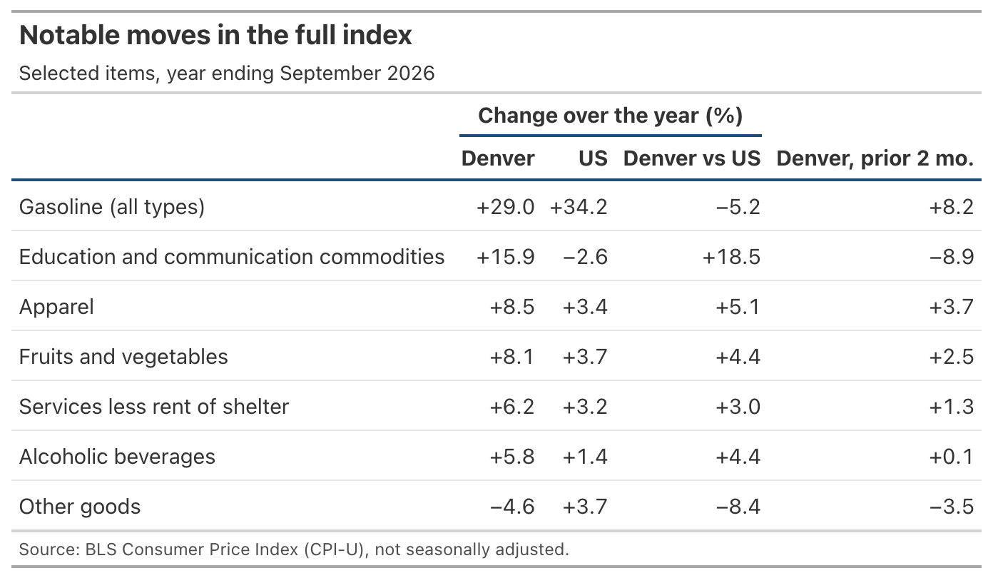Gas is at the top of the list of notable moves and I won’t spend much time on it other than noting that gas prices are up more than 8% in the two months since the July report.

Services less rent of shelter are up over 6% on the year and this is also 3 points higher than the U.S. average. This specific category includes things like insurance, medical care, childcare, phone, and internet services among others. Without additional details it’s difficult to say which specific services are contributing most to the rise but this is sure to hit many people’s budgets.

Similarly a few goods categories including apparel, fruits and vegetables, and alcohol are all up and well above the U.S. average. Time to eat more meat and drink less I guess.

Other goods are down 4.6% compared to 3.7% for the U.S. average. This category includes goods like tobacco, personal care, and other miscellaneous items. Although this appears as the one highlight of the report in terms of price relief, it very well could reverse in the next two months when the next report comes out. I wouldn’t bank on sustained price decreases in this area.

---

# Mayor Johnston on Childcare Costs in Denver

2026-07-29
Originally published on Substack: https://www.frontrangeeconomics.com/p/mayor-johnston-on-childcare-costs

![](/images/posts/mayor-johnston-on-childcare-costs/img1.png)

Last week, Mayor Johnston gave his [State of the City speech](https://www.youtube.com/live/n1aWyza3jzE) looking ahead to a possible second term. As [Paul Teske wrote](https://paulteske1.substack.com/p/affordable-denver) shortly after the speech, the major focus was on affordability in Denver. Within the bucket of affordability one of the highlights was childcare costs in Denver.

I recently wrote [a post here on childcare costs in Colorado](https://reillychandler.substack.com/p/the-cost-of-child-care-in-colorado) which covered what I see as three of the major causes of high childcare costs including cost disease, regulation, and the demand side. So, I was happy to see the Mayor putting a spotlight on this issue that parents all around the city are dealing with.

Mayor Johnston did not go into great detail in his speech but laid out a framework for a task force and policy changes intended to address childcare costs. Some of this sounds good but I don’t know how optimistic I am that it will bring about the desired changes. Part of this has to do with how the Mayor discussed childcare regulations.

The Mayor rightly points out that regulations are one of the things making it more difficult for providers to enter the market. But the way he describes this is “red tape” leading to providers drowning in paperwork. His exact quote was, “cut the red tape so passionate educators can open and run a quality childcare business without drowning in paperwork.” [Some work has shown that the fixed costs of compliance](https://www.cato.org/research-briefs-economic-policy/cost-regulatory-compliance-united-states) are significant. But I’m skeptical that direct compliance costs are the most costly part of the relevant regulations.

Even if the process of opening a daycare was streamlined (applications made easier, dealing with a single agency, etc.) such that “red tape” was cut, this wouldn’t mean constraints on child to staff ratios or other regulations suddenly became more flexible. I think a more serious look at regulations that goes beyond simplifying processes is warranted here. But I also don’t want to discount that even cutting paperwork would be an improvement.

My hope is that the task force looks into building some real flexibility into existing regulations. However, I am not even sure what they can achieve given that many of these regulations come from the state government. So, even if the Mayor’s plan was aimed at dramatic cuts in regulations, it’s not clear much could be done. Where there is room to create some regulatory flexibility at the city level, it should be pursued. And if that flexibility creates more options and allows for more entry without significant safety or other concerns that could be a major win toward the Mayor’s goals and may even encourage changes at the state level.

Another point on the topic of childcare in this speech was an idea for universal childcare in Denver. One version of this amounts to a subsidy for childcare along the lines of the city’s pre-K program. A subsidy will probably help people but will not directly address the supply problem the Mayor also pointed out. There is a large gap between how many daycare slots are available and how many children could fill those slots. Increasing demand while keeping supply constrained can just continue to push prices higher. But without specifics on what this would look like in Denver, I’ll save any further comments for when this comes out. It’s entirely possible there is a version of universal childcare that is a major help for Denver parents without creating a whole new set of problems.

---

# TABOR Doesn’t Care About Incidence

2026-07-14
Originally published on Substack: https://www.frontrangeeconomics.com/p/tabor-doesnt-care-about-incidence

![](/images/posts/tabor-doesnt-care-about-incidence/img1.png)

In 2020, Colorado voters passed [Prop EE](https://content.leg.colorado.gov/sites/default/files/initiative%2520referendum_2019-2020%20hb%2020-1427bb.pdf), increasing cigarette and tobacco taxes and joining the growing number of states that tax nicotine products commonly used as alternatives to tobacco and cigarettes. Although many states have implemented taxes specific to e-cigarettes, Colorado is (as far as I can tell) unique in that its nicotine products tax applies to “[any product that contains nicotine derived from tobacco or created synthetically that is intended for human consumption,](https://tax.colorado.gov/nicotine-products-tax-guide)” except for tobacco and cigarettes, which are taxed separately, and products such as nicotine gum or patches, which are considered cessation products. Even with those exceptions, the tax covers a wide variety of products including e-cigarettes and increasingly popular nicotine pouches such as Zyn. These products are subject to a percentage tax of the manufacturer’s list price, for which wholesalers and distributors are liable, that started at 30% when the law was implemented and increases to 62% by July 2027.

I’m hopelessly addicted to nicotine, so I have some personal (financial) reasons why I don’t like this tax. And as much as I might like to, I am not going to spend this post railing against it. Instead I am going to use it as an example to talk a bit about tax incidence and how Colorado is in a unique situation because of TABOR. The first two parts of this post will explain the basic economics of tax incidence and revenue. The incidence part will focus on how theory predicts and empirical work supports that for addictive products like nicotine, taxes are almost entirely paid by consumers. For similar reasons, we can also expect that for something like the broad category of nicotine products, a lot of tax revenue can be raised. But where I think this gets interesting is where TABOR comes in.

[Colorado’s TABOR](https://tax.colorado.gov/TABOR) (Taxpayer’s Bill of Rights) amendment to the state constitution is a complicated law, but one of its features is to set rules for how the state government must go about implementing new taxes. Among these rules is what happens when revenue from a new tax exceeds projections. The default is to refund the excess to taxpayers and lower the tax in proportion to the excess unless the question is put to voters who may allow the government to retain the excess revenue and keep the tax at the planned rate (note that this is different from the “TABOR refunds” on your state tax return). For the purposes of this post, whether that feature of TABOR is desirable or not in general is beside the point. The nicotine products tax is an interesting case of how TABOR can, in principle, create a situation where the legal taxpayers may receive a refund even if they did not bear the economic burden of the tax.

Revenues from the Prop EE taxes on nicotine products (along with increases in tobacco and cigarette taxes) were ultimately underestimated by more than \$20 million. As I argue in the rest of the post, this meant the taxes could have been refunded to suppliers rather than the consumers who bore most of the burden of the tax. But the legislature was able to put the question up to the voters in 2023, who favored allowing the government to retain the excess revenue and keep taxes on their planned schedule.

The taxes discussed here are an extreme example with nearly no overlap between the legal taxpayer and who actually paid. But the TABOR rule that defaults to refund the legal taxpayer means that there are likely many cases where a refund may go to those who only face a portion of the true economic cost of the tax.

### Tax incidence and the nicotine products tax

The simplified way to understand the idea of economic incidence is to compare the elasticities of supply and demand. Whichever side of the market is relatively less elastic will bear more of the burden of a tax. All this means is that whoever is less sensitive to changes in prices will bear more of the tax, regardless of who sends the money to the government.

When economists think about tobacco taxes, they point to the addictive nature of nicotine making consumer demand fairly inelastic. When cigarette prices increase, smokers don’t cut back that much. But cigarette producers can shift their supply away from high-tax areas fairly easily. So, smokers tend to bear a much larger share of the burden of tobacco taxes than producers. And this isn’t just an Econ 101 model and some assumptions. There is solid empirical evidence that smokers do in fact bear most of the burden of cigarette taxes.

A [2012 paper from Ryan Sullivan and Donald Dutkowsky](https://journals.sagepub.com/doi/10.1177/1091142112442742) that estimates the effects of local and state excise taxes on cigarettes finds evidence of more than full pass-through, meaning a \$1 increase in cigarette taxes raises the price of a pack of cigarettes by more than \$1. In [another paper from the same year by Matthew Harding, Ephraim Leibtag, and Michael Lovenheim](https://www.aeaweb.org/articles?id=10.1257/pol.4.4.169) using Nielsen Homescan data, the authors find cigarette taxes are less than fully passed through to pack prices (only about \$0.85 for every \$1 increase in taxes on average).

Although their results differ somewhat, the evidence supports the theoretical reasoning that smokers tend to bear a much larger share of the cigarette tax burden than producers.

I don’t have estimates of demand elasticity for broader categories like nicotine products, but when we think of consumer demand we can make some reasonable assumptions about when demand will be more or less elastic. Demand for Marlboro cigarettes will be more elastic than demand for cigarettes in general. Why? More substitutes generally means more elastic demand. Maybe there is some brand loyalty such that demand for Marlboro Reds would be less elastic than, say, demand for a particular brand of orange juice, but we should still expect that consumers will be *more* sensitive to price changes even for their favorite cigarette than for cigarettes in general.

One way to convince yourself of this is to consider how much pricing power Marlboro really has. Could they start charging \$25 for a pack of cigarettes and expect to lose only a few customers? Probably not. So, if we accept that consumer demand is typically less elastic the fewer substitutes there are, we can extend this to think about what that means for that broad category of nicotine products being taxed in Colorado.

The nicotine products tax encompasses a large share of cigarette substitutes that consumers may turn to, including vapes and nicotine pouches. If we compare demand for tobacco and demand for nicotine products, the intuition is that tobacco demand is more elastic than nicotine products demand simply because there are more substitutes for tobacco than there are for the category of nicotine products. If only e-cigarettes were taxed, we might expect substitution to nicotine pouches, but if both are being taxed at the same time, substitution doesn’t allow a consumer to avoid the tax.

The nicotine products tax in Colorado was not alone either. Tobacco and cigarette taxes were to increase under the same law. And because the taxes on substitutes like tobacco and cigarettes were also going to increase, we shouldn’t expect a large amount of substitution away from things like e-cigarettes and pouches to tobacco products (but maybe some substitution to the exempted medical products like nicotine patches). An additional implication is that we should expect the users of nicotine products to bear an even larger share of these taxes than tobacco users bear of tobacco taxes, unless there is reason to believe that the producers of nicotine products have systematically less elastic supply than tobacco producers, [which seems unlikely](https://www.9news.com/article/money/business/zyn-pouches-aurora-plant/73-6e740844-21d9-48be-a60b-48dba928726e).

### Tax revenue and the nicotine products tax

How the difference in elasticities affects incidence is not all that matters here either. We can also take this understanding of differences in elasticity on the demand side to make predictions about how much revenue may be collected from a tax.

If we assume some fixed elasticity of supply, the less elastic demand is, the more revenue will be raised for a given tax. The reasoning for who bears the burden of the tax is similar to why we expect more revenue with less elastic demand. When consumers are not very responsive to price increases (meaning they don’t reduce their consumption all that much), there is little change in quantity demanded between the pre-tax world and the post-tax world, and the government captures a portion of receipts for each sale.

For the sake of a simple example, assume that an increase in cigarette and nicotine product taxes completely passes through to consumer prices such that a \$1 increase in cigarette/nicotine product taxes increases the price of cigarettes/nicotine products by \$1. We can use this as a starting point to see how small differences in elasticity create big differences in how much revenue we expect a tax to raise.

Let’s say there is no tax in the market for cigarettes and the price of a pack is \$10. At this price, consumers purchase 1 million packs of cigarettes every month. The government introduces a \$1 cigarette tax, increasing the price to \$11 per pack.

If we want to make a prediction about revenue raised by this tax, we can use the elasticity of demand for cigarettes. Suppose we think the elasticity is -0.4, meaning that when prices increase by 10%, quantity demanded declines by 4%. So, under the \$1 tax (equivalent to a 10% increase in price), quantity demanded falls from 1 million packs per month to 960 thousand packs per month, and the government collects \$960,000 in tax revenue every month.

Now, we can do the same kind of example for nicotine products. The market price for nicotine products is \$10 before any tax and consumers purchase 1 million units monthly. Then, the government implements a \$1 tax on nicotine products, but now let’s say that the elasticity of demand for nicotine products is -0.2 (half that for cigarettes). The \$1 tax in this market reduces quantity demanded by only 2%, from 1 million units per month to 980 thousand. The government is able to collect \$980,000 in taxes in this market. The \$20,000 monthly difference in revenue becomes nearly a quarter million over the course of a year.

The sections on incidence and revenue give us two things to keep in mind: 1) Consumers pay more of a tax the more inelastic demand is (relative to the elasticity of supply); 2) Revenue raised from a tax will be higher the more inelastic demand is.

### TABOR and the nicotine products tax

Now that we know the basics of tax incidence and revenue, I can explain a weird possibility created by Colorado’s TABOR. I am not going to explain TABOR completely in this post (not sure I even could without reading much, much more about it), but one feature of the law that is relevant here is how new taxes are handled.

When the Colorado government implements a new tax and revenue collections exceed projections, the TABOR default is to refund excess revenue and reduce the tax rate unless voters approve a measure for the government to retain the excess and maintain the new tax rate. The legislature can introduce a ballot measure to seek voter approval on this.

Whether because no ballot measure is referred or because voters reject one, the excess revenue is refunded to whoever paid it to the government. But who pays the government tells us nothing about who bears the economic burden of the tax. So, a nicotine products tax levied on wholesalers and distributors but likely paid almost entirely by consumers could in principle result in revenue being refunded to the side of the market that didn’t bear the tax burden. That would be a windfall for the wholesalers and distributors.

Of course, this is only in principle, but voters were given this option a couple years after the Prop EE taxes went into effect. What happened? The Legislative Council Staff (LCS) is responsible for creating the revenue projections for new taxes in their fiscal impact statements. The [fiscal impact statement](https://content.leg.colorado.gov/sites/default/files/2020_fiscal_impact_statements_for_web.pdf) for the Prop EE cigarette, tobacco, and nicotine products taxes lays out how the LCS went about estimating revenue from the new nicotine products tax based on the limited data they had access to. And one assumption they made in their projections was that demand for nicotine products is more elastic than demand for cigarettes or other tobacco products. If what I am saying about the elasticity of nicotine products is true, then assuming more elastic demand than for cigarettes or tobacco would lead to an underestimate of revenue raised from nicotine products.

By the time the question reached voters in 2023, revenue had already come in above projections. The [fiscal impact statement from LCS for the Prop II ballot measure in 2023](https://content.leg.colorado.gov/sites/default/files/images/2_-_proposition_ii_-_fiscal_impact_statement.pdf) showed excess revenue of more than \$20 million and noted specifically that the “excess revenue was mostly due to tax revenue from nicotine products, such as e-cigarettes and vaping products.” Maybe the market for nicotine products grew more than expected because Zyn took off. Or maybe this was due to the data issues LCS notes in their initial fiscal impact statement. But I think the more likely story is that nicotine products were a less elastic market than LCS assumed and this led to more revenue being raised. It would be difficult to differentiate between unexpected market growth and the elasticity issue as contributors to the excess revenue. But the elasticity story makes more sense to me in part because the revenue estimate LCS used assumed 3-8% market growth, which is fairly large on the upper end.

To be fair, I am not arguing that the LCS made an obvious error. They were dealing with incomplete data on top of uncertainty about how the nicotine products market might evolve, among other things. This uncertainty is explicit in the fiscal impact statement, where LCS notes, “the market for nicotine and vaping products is expected to continue to evolve in coming years, and the pace of increasing consumption is expected to slow as federal, state, and local regulations on the industry tighten.” Their assumption about demand for nicotine products is not unreasonable either. If I had to guess, they were probably assuming that e-cigarettes make up the largest portion of this market, and I was able to find at least [one empirical estimate of e-cigarette demand elasticity](https://tobaccocontrol.bmj.com/content/34/1/34) that is close to the number LCS used. But it’s hard to say for sure without knowing more about what went into their methodology. These are tough predictions to make, and it is easy in retrospect to point out one area that is a plausible culprit for a missed projection.

Ultimately, voters (by a strong margin) chose to allow the government to retain the excess revenue and keep the taxes in place. Wholesalers and distributors did not get their windfall. But that may not always happen. This TABOR rule doesn’t care about incidence.

---

# The Cost of Child Care in Colorado

2026-07-06
Originally published on Substack: https://www.frontrangeeconomics.com/p/the-cost-of-child-care-in-colorado

Over the last few weeks, I have not been posting as much because of a pretty big life change. My daughter was born at the end of May and most of my attention has been on her and my wife at home. We are fortunate enough to both have substantial time off from work to be at home with the baby but soon enough we will be facing the problem that most working parents face. How are we going to adjust to the looming childcare expense?

Working parents around the country, especially those without extended family to lend a helping hand, are faced with difficult financial choices when it comes to finding childcare. According to data from a [report published by the Common Sense Institute](https://www.commonsenseinstituteus.org/colorado/research/jobs-and-our-economy/the-child-care-opportunity-index), average monthly childcare costs in Denver are \$1,574 and Boulder County tops the state’s most expensive counties with average monthly costs over \$1,600. Compare these average costs to average wages in Denver and parents are spending 18% of their paycheck on childcare and even more in other Colorado counties.

![](/images/posts/the-cost-of-child-care-in-colorado/img1.png)

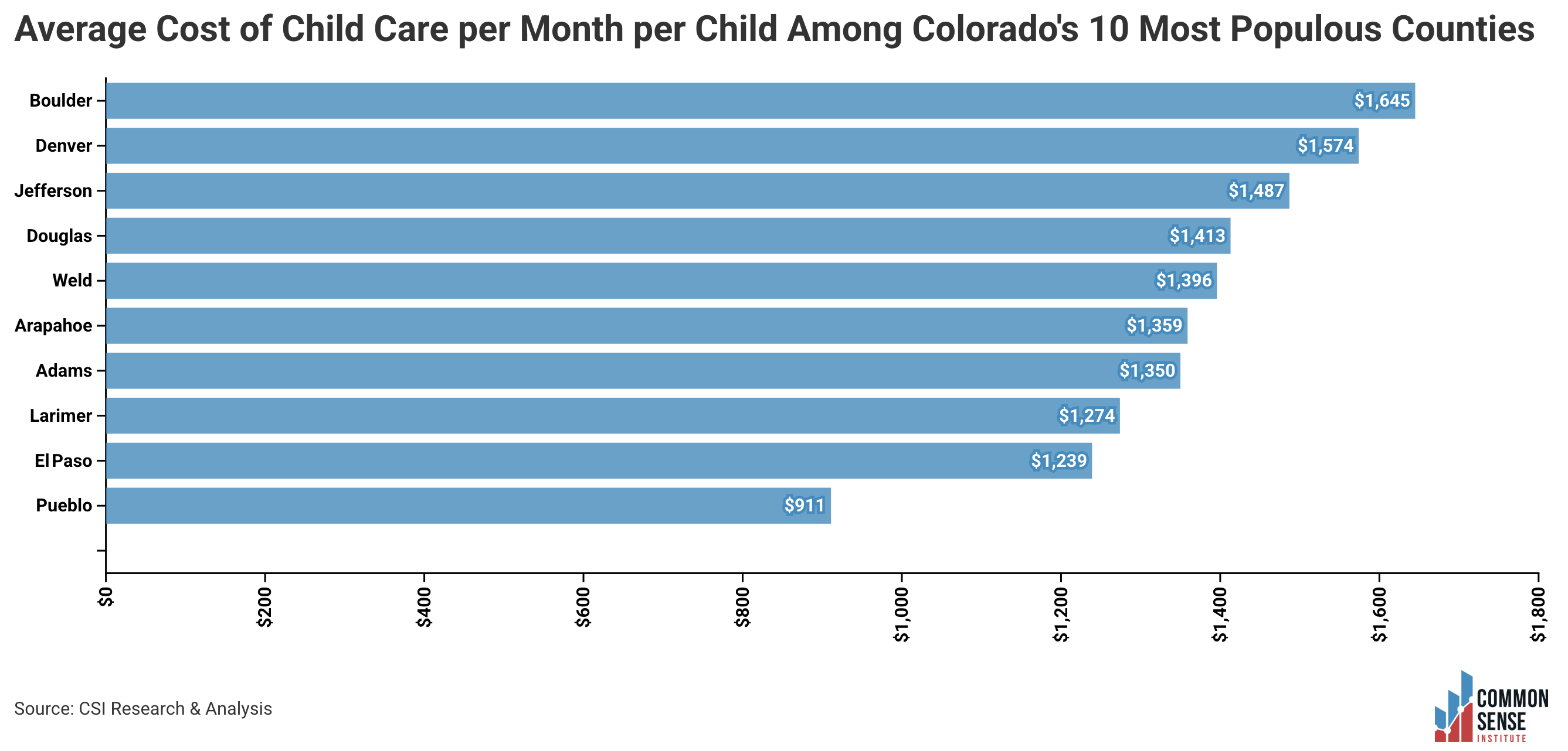
The financial difficulties extend to providers as well. The [Colorado Sun recently covered](https://coloradosun.com/2026/06/29/boulder-county-early-childcare-costs/) how providers like a daycare in Boulder operate on increasingly thin margins despite rising costs for parents. Leadership within the daycare quoted in the Colorado Sun article emphasizes that many of these difficulties stem from declining government support such as the freeze in the Colorado Child Care Assistance Program.

I think few would disagree that rising childcare costs pose a problem for working families but there is considerable debate over what is causing it and what can be done about it. What I want to focus on here are a few explanations for why these costs are so high in the first place. The first is the “Baumol effect” or “cost disease.” Second is how regulations, looking specifically at Colorado, can increase costs. And lastly I’ll offer a less often discussed factor on the demand side.

### The Baumol effect

The Baumol effect or cost disease idea goes back to the economist [William Baumol](https://en.wikipedia.org/wiki/William_Baumol), who developed a straightforward theory to explain how differences in productivity growth across sectors of the economy could result in diverging costs and ultimately prices of outputs. I’ll give my simplified retelling of the theory.<a href="#footnote-1" id="footnote-anchor-1" role="doc-noteref">1</a> Start by assuming there are two sectors in the economy, the goods producing sector and the services sector. In the goods producing sector, labor productivity can be easily augmented with capital or technology and in the services sector, which is more labor-intensive, productivity remains relatively constant, largely unaffected by increasing capital and technology. Rising productivity in the goods producing sector pushes up wages there. But if workers in the service sector can move between sectors, they won’t just ignore the opportunity for higher wages. And this could mean fewer workers in the service sector to produce output if employers do nothing. What can employers in the service sector do to try and keep workers? They can offer higher wages to workers to keep them around, even though there has not been much rise in productivity. When input costs (like workers’ wages) rise without a corresponding increase in productivity, relative prices must rise and output may fall.

Childcare is a labor-intensive service, so Baumol’s theory might help explain its rising costs. You need people around to take care of all those kids and there’s really not much machines or technology can do to change that (yet?). We should then expect that for the childcare industry to keep workers it must pay them more. The theory does not predict that childcare workers are making great money, only that their wages are growing over time relative to their productivity growth. A simple comparison to see if we have evidence in favor of the Baumol effect for childcare is to look at growth in average wages in childcare compared to growth in average wages for all private industries as shown in the chart below for Denver County going back to 1990. Average wages in childcare have shown a more than 5x increase over the period while average wages in all private industry have gone up about 4x. Childcare costs are high and wages are growing, so Baumol’s theory is probably part of the story here. But that doesn’t mean this theory can completely explain why childcare costs are so high.

![](/images/posts/the-cost-of-child-care-in-colorado/img2.png)

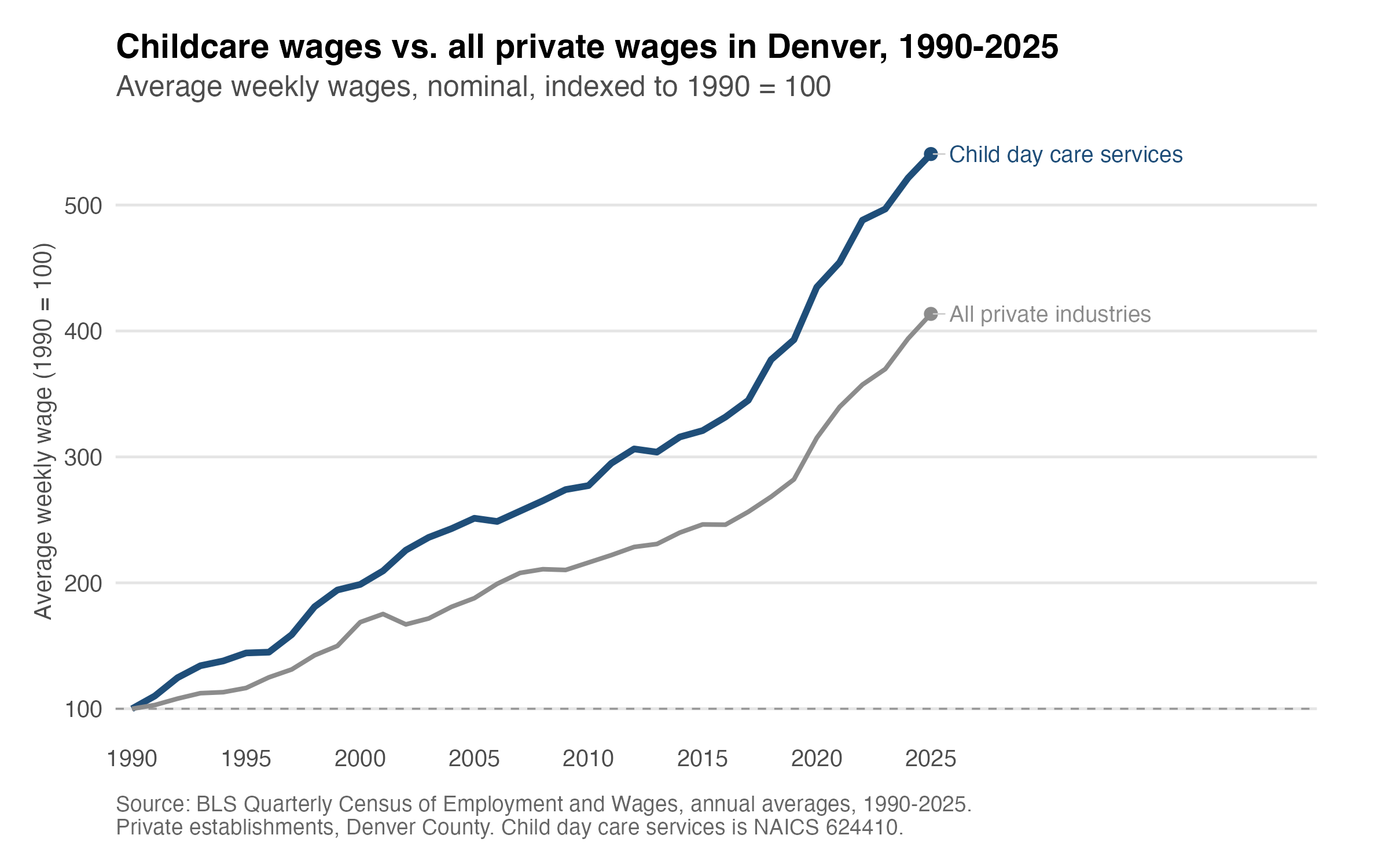
### Childcare regulations

Another factor that contributes to high childcare costs is regulation. Childcare regulations include restrictions on daycare facilities like how many square feet of indoor space per child or fence heights for outdoor areas. They also include thresholds for child-to-staff ratios and licensing requirements for operators and staff. The [Archbridge Institute has a state-level dataset](https://www.archbridgeinstitute.org/state-childcare-regulations-database/) that provides useful details on these sorts of regulations. [Colorado is about average](https://www.archbridgeinstitute.org/wp-content/uploads/2026/02/2026-State-Childcare-Regulations-Index.pdf) on the strictness of its childcare regulations.

Depending on their stringency, these regulations can restrict supply and put upward pressure on operating costs. How much this is contributing to the rising costs of childcare is up for debate. [Alex Tabarrok has written](https://marginalrevolution.com/marginalrevolution/2025/07/the-rising-cost-of-child-and-pet-day-care.html) that the Baumol effect likely dominates by comparing rising costs in the more heavily regulated childcare sector to those in the lightly regulated pet daycare sector. But some regulations specific to childcare can also interact with the Baumol effect. Take child-to-staff ratio regulations.

Colorado, like many other states, varies its child-to-staff ratios by age. The ratio is lowest for the youngest groups with 5 children per staff member from ages 0 through 2.5 years. That number jumps up to 8 for 2.5 to 3 year olds and then all the way up to 15 for 7 to 8 year olds. Suppose we have a daycare for children 0 to 2.5 years old that is about to open. The daycare has 10 children signed up for the coming month and must have at least 2 staff members to meet these regulatory thresholds. If the daycare is to sign up just one more child, it would have to hire another employee or risk being in violation of the regulation. Even at the state minimum wage of \$15.16/hour, an additional full-time employee creates more than \$2,400/month in additional labor costs. Either enrollment must be capped or the daycare charges enough to at least cover labor costs.

It is not that these child-to-staff ratios are unreasonable. I certainly wouldn’t want to send my daughter to a daycare where one employee is trying to take care of a dozen infants and toddlers by themselves. But these thresholds create hard cutoffs that reduce the flexibility of care centers. That lack of flexibility can increase operating costs and contribute to higher prices. But higher prices are not just a matter of operating costs, we need to look at the demand side as well.

### Demand for childcare

Like I said above, regulation or not, I wouldn’t send my daughter to a daycare that couldn’t give her the time and attention I thought was necessary for her to be happy and properly cared for. I am not alone there either. Most if not all parents feel similarly and I don’t think it stops there. Maybe part of the rising cost of childcare is not cost disease or regulation but a rise in quality that people are paying for.

It is not exactly fair to say that this demand story is totally unrelated to the cost disease. As [Tyler Cowen points out in a 1996 comment](https://link.springer.com/content/pdf/10.1007/BF00153847.pdf) on Baumol, there is an optimistic version of the cost disease argument in Baumol’s own work. Rising productivity in some parts of the economy increases the opportunity cost of production in the less productive parts (the arts in his case, childcare here), so prices rise and output may fall. But rising productivity also means rising incomes. As incomes rise, people are willing to pay for services like childcare even at higher prices, so output may not fall and could even increase. Cowen then goes further and argues against the cost disease in the arts altogether. The arts were never stagnant, he says. The arts kept improving, so comparing the cost of a performance today to one decades ago is comparing apples to oranges. Part of what looks like the same thing getting more expensive is people paying for a better thing. A version of that argument applies to childcare too.

Parents have gotten richer, and I believe that shows up in two ways here. They are willing to pay more for childcare, and they are willing to pay for a higher quality version of it. You can see the second one all over the Denver area. [La Petite Academy](https://www.lapetite.com/area/denver-aurora/), a national chain of childcare centers with several locations in Denver’s surrounding counties, streams live video of the classroom to parents, provides [mathematics in their early preschool curriculum](https://www.lapetite.com/educational-programs/curriculum/early-preschool/), and boasts [dedicated adult attention for infants](https://www.lapetite.com/educational-programs/curriculum/infants/) through an assigned primary caregiver. [The Gardner School](https://www.thegardnerschool.com/schools/the-gardner-school-at-9co/) in Denver sends [real-time updates through a parent app](https://www.thegardnerschool.com/blog/communication-with-parents-helping-you-stay-connected-to-your-child/) and emphasizes [research-based S.T.E.A.M. activities](https://www.thegardnerschool.com/blog/a-look-at-steam-learning-at-the-gardner-school/). The Gardner School even offers [enrichment programs for children as young as two](https://www.thegardnerschool.com/twos/) with options like dance, karate, music, cooking, computers, and foreign language. If you want to start foreign language learning for your child even sooner, [Denver International Schoolhouse](https://dispreschool.com/) in Aurora will start your infant on Spanish immersion. These are just a few examples from a quick search of additional services beyond basic childcare offered by many providers.

Much of this was not on the menu a generation ago or at least available to the extent it is now. So even if parents today buy about the same hours of care each month as parents did 30 years ago, comparing cost per hour over time is not comparing the same product. But this raises a question. If some of these quality improvements like the live streaming and apps are technology based, why would this make childcare more expensive? Notice that many of these quality upgrades still lean heavily on labor. The language immersion, the STEM classes, the enrichment programs all require people, and people whose time is not easily augmented with capital or technology. These kinds of quality improvements are expensive to provide and are not the same product as basic childcare. Even if the examples I listed capture only part of the market (the more expensive end), this will still be part of the rise in average costs. Although it is likely that basic childcare is getting pricier, parents are also choosing to buy a higher quality version.

### Conclusion

Childcare is expensive and likely will continue to be that way. Perhaps easing some of the more stringent regulations can help. One candidate would be licensing exemptions or lighter requirements for smaller daycares, say something like 10 children or fewer. Under current [Colorado law](https://drive.google.com/file/d/1A3RO-zH7GpuMHn5-LP97Biq3MgUwfJ4E/view?usp=sharing), child care licenses are required for any regular care of more than four children or more than two children under the age of two. If you have two kids and want to hire a nanny, the nanny doesn’t need to be licensed. But if you and a couple of neighbors, each with two kids, wanted regular care provided by one parent who stays home or to split the cost of a couple nannies, then a license is necessary.

A broader exemption or lighter requirements (along the lines of [this suggestion from Kelsey Piper](https://x.com/KelseyTuoc/status/1902821324105699642)), not necessarily completely unregulated, could open up the possibility for a daycare analog to homeschooling pods or “microschools” that became more popular during and since the pandemic. No one bats an eye at having your friends or neighbors watch your kids or hiring a nanny on your own, so why not create a more conducive environment for families of young children to create daycare pods or something similar?

A daycare pod doesn’t get around the issue of childcare being labor intensive, but it creates some flexibility not allowed by current regulations. And because pods are small and more individualized, they may be able to more easily meet the idiosyncratic demands of families in different communities. On the cost side, [expanding supply should ease some of the upward pressure on prices](https://edwardjtimmons.substack.com/p/why-child-care-regulatory-reform). And it seems easier to work out [alternative arrangements among families](https://www.minneapolisfed.org/article/2025/who-do-parents-call-when-professional-child-care-is-out-of-reach) to share responsibilities or otherwise reduce the financial hit associated with traditional childcare.

<a href="#footnote-anchor-1" id="footnote-1" role="doc-backlink" aria-label="Back to reference 1">1</a>

For Baumol’s original paper see [here](https://www.jstor.org/stable/1812111). For a more recent treatment and application of Baumol’s ideas to different services see [Eric Helland and Alex Tabarrok’s book](https://www.mercatus.org/system/files/helland-tabarrok_why-are-the-prices-so-damn-high_v1.pdf).

---

# The Creation of the Rocky Mountain Arsenal National Wildlife Refuge

2026-09-14
Originally published on Substack: https://www.frontrangeeconomics.com/p/the-creation-of-the-rocky-mountain

<img src="/images/posts/the-creation-of-the-rocky-mountain/img1.jpeg" alt="" width="1456" height="1092">

*Bison along the wildlife drive at Rocky Mountain Arsenal National Wildlife Refuge. Photo by the author.*

*Note: This post may be cut off in your email. Click the title to read directly on Substack or in the app.*

When I moved to Denver, one of the first outdoorsy things I did was visit the [Rocky Mountain Arsenal National Wildlife Refuge](https://www.fws.gov/refuge/rocky-mountain-arsenal). “Outdoorsy” being used extremely loosely here since I only did the wildlife drive. Having spent most of my life in Southern California and a few years on the East Coast, being able to see bison up close just a short drive from my new home was a pretty cool experience. I don’t know how people who grew up around here feel about the refuge. Maybe it’s considered weak as far as nature sights go in the area or just a spot for tourists. But since my first time going it’s been somewhere I take family and friends who are visiting.

I came across the Arsenal by accident while working on a paper in my last semester of graduate school. My advisor had been asked to contribute to a special issue on defense economics and came to me to co-author a paper. I had been thinking about this idea on military base closure and we began working.<a id="footnote-anchor-1" href="#footnote-1" role="doc-noteref">1</a> In doing research for that project, I read an article discussing the creation of the Arsenal refuge. That paper, “[From Weapons to Wildlife: The Transformation of the Rocky Mountain Arsenal](http://dx.doi.org/10.1080/00139159809604586),” by Karen Wiley and Steven Rhodes, will serve as one of the main sources I draw from for this post.

The 27 square miles of land just outside Denver that is now a wildlife refuge (most of it anyways) was an Army chemical weapons plant also used by Shell Chemical to produce pesticides for decades. The site itself was heavily polluted with toxic waste from all the chemical production. Then during the 1950s some adjacent farms suffered crop damage and later it was discovered that pollutants had made their way into the groundwater offsite. The Colorado state government, the Army, and Shell Chemical spent years in legal disputes over who was going to clean up all the pollution, who was going to decide the cleanup standard, and how that land might be used in the future. Then, bald eagles were found roosting on Arsenal land, and that discovery kicked off a series of events leading to the designation of the Arsenal as a wildlife refuge.

In this post, I am going to explain how these events unfolded through the lens of the bootleggers and Baptists theory of regulation. The Army and Shell represent the bootleggers, who were responsible for cleanup costs and had an interest in keeping those costs as low as possible. Colorado wanted to set cleanup standards at a level higher than the Army or Shell wanted to pay. It wasn’t until bald eagles were discovered on the Arsenal that the opportunity to lock in land use as open space or refuge was a realistic possibility.

That possibility was appealing to some environmental groups, our Baptists, who could rally public support for turning the old weapons plant into a safe haven for wildlife. But it was also appealing to the Army and Shell as cleanup standards for a refuge would be much lower than almost any other use. And so we have the conditions for our bootleggers and Baptists to work together toward their common goal of creating a wildlife refuge. I’ll start by explaining a bit more about the bootleggers and Baptists theory.

### The bootleggers and Baptists theory

The bootleggers and Baptists theory of regulation comes from [Bruce Yandle’s 1983 paper](https://access.heinonline.com/HOL/P?h=hein.journals/rcatorbg7&i=122) published in the journal *Regulation*. [In a later 1999 paper](https://access.heinonline.com/HOL/P?h=hein.journals/rcatorbg22&i=127), Yandle summarized his theory as follows:

> \[D\]urable social regulation evolves when it is demanded by both of two distinctly different groups. “Baptists” point to the moral high ground and give vital and vocal endorsement of laudable public benefits promised by a desired regulation. … “Bootleggers” are much less visible but no less vital. Bootleggers, who expect to profit from the very regulatory restrictions desired by Baptists, grease the political machinery with some of their expected proceeds.

His summary is clear but I think Yandle’s idea is best captured in the simple story that gives the theory its name. Here’s my version of it:

Suppose legislation is proposed in a county to prohibit liquor stores from being open on Sundays. The days of Prohibition are far behind us, but it is easy to imagine that there may be some groups, such as Baptists, that support this law on moral grounds. Sure, they might prefer alcohol to be illegal, but closing liquor stores on Sundays is still a win.

The advantage for the Baptists is their ability to rally public support for their cause. You and your neighbors want to look like good Baptists who would keep the county’s residents from being tempted by drunkenness on Sundays. Baptists won’t be alone in supporting this law, however.

Some groups, such as bootleggers, have an economic interest in restricting the operating hours of liquor stores. If liquor stores are closed on Sundays, that is one day a week with less competition for the bootleggers. The problem is bootleggers will find it much harder to drum up public support for their position. Luckily for them, they want the same thing as the Baptists who *can* drum up that support.

Since Yandle’s contribution, there have been [many](https://access.heinonline.com/HOL/P?h=hein.journals/yjor33&i=315) [applications](https://access.heinonline.com/HOL/P?h=hein.journals/rcatorbg31&i=100) [of](https://www.jstor.org/stable/48617481) [the](https://doi.org/10.1007/s11127-020-00822-5) [theory](https://doi.org/10.1007/s11127-023-01123-3) from other scholars, [extensions](https://doi.org/10.1007/s11127-026-01376-8), and a [formal model](https://doi.org/10.1007/BF00714398) that captures the dynamics of bootlegger and Baptist behavior including when bootleggers are willing to pay Baptists. Although bootleggers and Baptists need not directly coordinate, the common thread through all this research is that their shared cause increases the chance of success and may create incentives for coordination.

At the Arsenal, the dispute was over who was liable for the environmental cleanup caused by decades of chemical pollution and who would decide how much cleanup should be done. The Army and Shell Chemical represent the bootleggers whose interests were in minimizing the costs of environmental cleanup. They were against the state of Colorado, which wanted to enforce a higher state standard that could have cost the Army and Shell billions more than they hoped to spend. The Army and Shell both fought in court to limit those costs with mixed results. It wasn’t until a Baptist case for lower levels of cleanup could be made that the two got what they wanted. Before I talk about how that happened, it will be helpful to understand more of the background of the Arsenal and the disputes surrounding cleanup.

### Brief history of the Arsenal site

The Rocky Mountain Arsenal was originally constructed in 1942 as a chemical weapons production facility. [Reporting on the facility from 1943](https://www.coloradohistoricnewspapers.org/?a=d&d=RMD19430403-01.2.115) suggests that goings-on at the Arsenal were initially shrouded in secrecy, though it was generally known “war gas” was being produced there. In April of 1943, John Stephenson of The Rocky Mountain News took an Army guided tour of the facility and was given a firsthand look at the large-scale production of mustard gas and Lewisite to be used during World War II.

<img src="/images/posts/the-creation-of-the-rocky-mountain/img2.jpeg" alt="" width="146" height="433">

*“Dressed Up”: John Stephenson, Rocky Mountain News writer, as the Army dressed him up for his inspection trip through Rocky Mountain Arsenal. U.S. Army Signal Corps photo, [Rocky Mountain News, April 3, 1943, p. 17](https://www.coloradohistoricnewspapers.org/?a=d&d=RMD19430403-01.2.115), via the Colorado Historic Newspapers Collection.*

The Army continued to produce chemical weapons at the Arsenal for the next couple of decades, including napalm and sarin. But even as the facility ramped down weapons production at the end of World War II, part of the land and facilities was leased to a private company that was eventually acquired by Shell Chemical (part of Shell Oil). Starting in the early 1950s, Shell used the site to produce pesticides and herbicides. Shell’s use continued for the next 30 years until the end of its lease in 1982.

<img src="/images/posts/the-creation-of-the-rocky-mountain/img3.jpeg" alt="" width="291" height="488">

*“Here’s the Way It Works”: Maj. Frank Chrencik demonstrates the chlorine cell to newspapermen during their visit to Rocky Mountain Arsenal. U.S. Army Signal Corps photo, [Rocky Mountain News, April 3, 1943, p. 17](https://www.coloradohistoricnewspapers.org/?a=d&d=RMD19430403-01.2.115), via the Colorado Historic Newspapers Collection.*

As you might imagine, decades of producing chemical weapons, pesticides, and herbicides, as well as the destruction of unused chemical weapons, created enormous amounts of toxic waste. Much of this waste was stored in man-made ponds on the Arsenal. After production of both weapons and industrial chemicals ended on site, the toxic waste didn’t just disappear. The waste ponds, like Basin F, were still filled. Buildings were contaminated. And the land itself had accumulated toxins. However, not all the toxic waste remained within the boundaries of the Arsenal.

As early as the 1950s there was some evidence of pollution from the Arsenal making its way offsite as farmers faced crop damage, according to Wiley and Rhodes. But it wasn’t until the 1970s that the state of Colorado became more involved. [The Rocky Mountain News reported](https://www.coloradohistoricnewspapers.org/?a=d&d=RMD19750403-01.2.14) early findings in 1975 of a “substance known as DIMP, a by-product of the detoxification of nerve gas” that officials from the Colorado Department of Health had identified in a few “water wells on and north of the Army’s Rocky Mountain Arsenal.” At the time, there was uncertainty surrounding the toxicity of DIMP, but the findings worried state officials about the full extent of pollution spreading to surrounding land. These findings marked the beginning of legal disputes between Colorado, the Army, and Shell.

### The state of Colorado vs. the Army vs. Shell

Almost immediately after the DIMP discovery, the Colorado Department of Health sent the Army and Shell three administrative orders: 1) stop discharging DIMP, 2) clean up its sources, and 3) start monitoring the groundwater. Rather than spend a few thousand extra words describing in great detail the administrative orders, lawsuits, and appeals that unfolded over the nearly two decades between the 1975 DIMP findings and the eventual creation of a wildlife refuge, I am going to limit this to the broad strokes. The three actors of interest at this point in the story are the state of Colorado, the Army, and Shell.

After the Colorado Department of Health discovered DIMP offsite in 1975, Colorado was intent on enforcing state law to hold the Army and Shell financially responsible for cleanup and to have the state, rather than the federal government, set the cleanup standard for the Arsenal. The state wanted an unrestricted-use cleanup standard enforced through Colorado’s hazardous waste law. The state’s position was further solidified as additional offsite contamination was discovered into the early 1980s and Colorado sued the federal government to force it to comply with state authority over cleanup standards.

The Army, on the other hand, wanted to keep cleanup standards and control with the federal government. From the Army’s perspective, much of the Arsenal was already a Superfund site and so belonged under federal law enforced by the EPA. As part of the strategy to achieve federal control in court and in direct response to Colorado’s suit to enforce the state’s hazardous waste law, the Army nominated the Basin F waste pond on the Arsenal to the National Priorities List. Their thinking was that by adding another piece of the Arsenal to the National Priorities List, the EPA’s role in determining cleanup would be solidified. At the same time, the Army wanted Shell to pay for part of the cleanup given the company’s share of the contamination. To this end, the Army sued Shell for cleanup costs. Shell then decided to sue its insurers to have them pick up the bill for any cleanup costs it might be found liable for.

The Army and Shell had pure economic interests in the cleanup costs and did as you might expect. The initial strategy for both parties was to rely on the courts to figure things out. For the Army, maintaining federal control would make it more likely cleanup standards would be lower, and so cheaper. Shell’s hope was a successful suit against its insurers to save on cleanup costs. This strategy proved mostly unsuccessful for the Army and Shell, and it was also incredibly slow.

Despite the sluggish process, in 1984, the Army announced its selection of a \$357 million cleanup option focused on what Wiley and Rhodes describe as “consolidation of all contaminated materials in a permanent on-post disposal site.” A year after the Army selected a cleanup option, a district court ruled that the Army and Shell were liable for the environmental damage. This didn’t mean that the state of Colorado would get the level of cleanup it wanted but did solidify who would be financially responsible for the cleanup. Now the uncertainty was over what level of cleanup (and therefore what the cost would look like) was going to happen at the Arsenal.

While all this was going on, the potential for developing land on and around the Arsenal drew additional interests into the central dispute over cleanup. State and city governments, including Denver and Commerce City, were involved in the development of the E-470 highway and a new airport (what is now DIA). Commerce City also saw an opportunity for the development of Arsenal land for commercial or residential purposes. These groups, though not directly involved, had a stake in the success of the state’s case. A higher cleanup standard with the Army footing the bill would open up opportunities for new sources of tax revenue and investment for local developers without the difficulty of figuring out how to fund what could be a multibillion-dollar cleanup.

Something to keep in mind about the cleanup standards dispute is that it is difficult to separate it from questions over future land use of the Arsenal. Colorado’s position was that it wasn’t interested in determining land use. But cleanup standards under the law Colorado was hoping to enforce, like its federal counterpart, are determined by potential risks to people on the land. Those risks are related to expected use, as was recognized by the development interests discussed above. So, we can’t really separate Colorado’s position or the Army and Shell’s positions over cleanup standards from expectations over future use of the Arsenal. Wiley and Rhodes explain how their respective positions were related to land use expectations:

> \[Colorado\] had adopted the position that the arsenal should be clean enough to support relatively unlimited human use, perhaps even residential use. … In contrast, the army and Shell had come to support a selective remediation policy that included on-site pollution containment and treatment. This assumed continued restrictions on public access to and use of arsenal property.

As long as the land use question for the Arsenal remained open, Colorado could fight for the unrestricted-use cleanup standard. If anything were to settle the future of how the Arsenal would be used, particularly if use was restricted, the Army would be more likely to get what they wanted. Then in late 1986, bald eagles were discovered on the Arsenal. It was this discovery that eventually settled the land use question.

### The bald eagles discovery

<img src="/images/posts/the-creation-of-the-rocky-mountain/img4.jpeg" alt="" width="492" height="423">

*U.S. Fish and Wildlife biologist Pete Gober measures the wingspan of a bald eagle captured on Rocky Mountain Arsenal. Photo by Wendy Shattil and Bob Rozinski, [Rocky Mountain News, December 25, 1988, p. 8](https://www.coloradohistoricnewspapers.org/?a=d&d=RMD19881225-01.2.24), via the Colorado Historic Newspapers Collection.*

The discovery of bald eagles at the Arsenal brought another government agency into the picture, the U.S. Fish and Wildlife Service (FWS). Bald eagles are “not just any endangered species” but “the national symbol and the longest-standing entry on the list of endangered species,” as Wiley and Rhodes put it. And under U.S. law they are protected not only by the Endangered Species Act but also by the 1940 Bald Eagle Protection Act. The combination of these laws and the fact that the birds were discovered on federal land meant that FWS (quoting Wiley and Rhodes again) “had jurisdiction to take virtually any action it deemed necessary” until the agency figured out what the eagles were doing on the land. As a result, “any activity that might disturb the raptors’ activities was effectively prohibited.”

Some wildlife officials, though uncertain about how regularly the eagles were using the roost at the Arsenal, saw the opportunity for something like a refuge. Pete Gober of FWS was quoted in the [Aspen Daily News in 1987](https://www.coloradohistoricnewspapers.org/?a=d&d=ADN19871215-01.2.32) as saying, “If this place could be cleaned up, it could be an amazing urban wildlife area. Amazing.”

The state of Colorado, the Army, and Shell at this point still held their initial positions. But as sociologist Melissa Lynne Hippard explains in [her dissertation on the Rocky Mountain Arsenal](https://www.proquest.com/dissertations-theses/consensus-making-state-nature-case-rocky-mountain/docview/304857795/se-2), the bald eagles “increased the level of interest by wildlife organizations” and “provided a conceptual end use that was federal in status and would satisfy local interest in open space preservation.” As wildlife protection became a clearer priority, the Army and Shell took advantage of the situation.

### Bootleggers and Baptists coordinating directly

Much of the interest in wildlife preservation on the Arsenal began with FWS working in conjunction with groups such as the National Wildlife Federation (NWF) and the Denver chapter of the Audubon Society ([an organization focused on protecting birds and their habitats](https://www.denveraudubon.org/about-us#OurMissionVision)). Together they focused on figuring out how preservation could be achieved and found strong public support for the idea. The entrance of these new interests into the land use question at the Arsenal was good news for the Army and Shell. Rebecca Cantwell, writing for [The Rocky Mountain News in 1988](https://www.coloradohistoricnewspapers.org/?a=d&d=RMD19881225-01.2.24), put the Army and Shell’s position plainly, writing that they “want a less intense cleanup and support the open space plan.”

Almost as quickly as FWS began their involvement at the Arsenal, Shell and the Army saw the agency and wildlife organizations as allies. If the Arsenal land were to be designated a refuge it would be more likely that cleanup standards would be lower (because of less human use), making cleanup cheaper than if alternative land use options remained a possibility. Shell was quick to put on its Baptist hat before working with groups like NWF and independently hired wildlife photographers to take pictures of animals found across the site. Shell acting on its own in this way may have helped build support for the preservation option, but it would be easy to see through their efforts as a mask for the true interest in lowering cleanup costs. Hippard quotes an anonymous FWS employee who appeared to be thinking along these lines:

> I believe Shell and (the) Army looked at it and wondered would it be a little cheaper for us to cleanup to refuge and wildlife standards instead of residential standards.

Shell could do better by coordinating directly with the organizations involved in preservation efforts. According to Hippard, the National Fish and Wildlife Foundation worked with Shell to get money to Denver Audubon to help build public support for turning the Arsenal into a wildlife refuge. Denver Audubon used this money to run public tours of the Arsenal (the Army still controlled access), sell wildlife calendars, and send letters to Congress. Coordinated efforts continued with Bald Eagle Days, events sponsored by the Army and organized by FWS and volunteers from Audubon, which brought thousands of people onto the Arsenal.

Hippard goes on to explain how central the bald eagles were to the efforts to build public support. The Army went as far as working with the Colorado Division of Wildlife and the Colorado State Patrol to bring animal carcasses onto the site when a plague swept through the eagles’ primary food source, prairie dogs. Keeping the eagles around was paramount to solidifying popular support through continued viewing opportunities and making the Arsenal a known location for wildlife viewing just a short drive from Denver. The bootleggers and Baptists dynamic that was emerging seemed to have been recognized by those involved. For example, Hippard quotes an anonymous member of a wildlife organization referring to the “unholy marriage” of “environmental interests and Army and Shell’s interests.”

The first piece of concrete progress toward the Arsenal becoming a wildlife refuge was a Federal Facilities Agreement signed in early 1989 designating “significant portions” of the site as available for use as open space. This was not a permanent designation and Colorado refused to sign on, but it was a formal move in the direction of taking land development options off the table. As these efforts continued and public support for the refuge option grew, the next step was to lobby for legislation. In typical bootlegger fashion, it wasn’t going to be strategically sound for the Army and Shell to take the lead on pushing for refuge designation by the federal government. If they were to get the cheaper cleanup they desired, they needed to rely on another coordinating actor to give the Baptists a stronger voice in the process.

Colorado Representative Pat Schroeder took on that role. Schroeder, encouraged by the NWF, introduced an amendment to the 1990 defense spending bill in the House that would designate the Arsenal as a national wildlife refuge and cap cleanup at the level from the 1989 agreement. This proposal would satisfy the Baptists with a refuge and the bootleggers with a cap on cleanup. But the amendment eventually failed after being met with substantial opposition over the cleanup cap.

One of the most vocal opponents of Schroeder’s amendment was another Colorado politician, Senator Tim Wirth. Wirth was adamant that [Colorado should have the authority to set higher cleanup standards at the Arsenal](https://www.coloradohistoricnewspapers.org/?a=d&d=RMD19891102-01.2.45). From Schroeder’s point of view, dragging the already long fight on even longer was going to waste money and risk Colorado losing access to federal cleanup funds. At the time the amendment failed in 1989, [The Rocky Mountain News reported](https://www.coloradohistoricnewspapers.org/?a=d&d=RMD19891102-01.2.45) that estimated cleanup costs for the Arsenal were between \$1 billion and \$4.5 billion. And the article goes on to say that Wirth and Colorado Governor Roy Romer acknowledged meeting state cleanup standards would be more expensive. However, for Wirth the issue was enforcing state law, not worrying about how much the Army might have to pay to comply. Schroeder, in contrast, seemed to recognize the need to compromise on cleanup standards to achieve an end use for the Arsenal that many supported.

That the opposition was largely focused on removing the cleanup cap language from the legislation ended up working in Schroeder’s favor. The end use for the Arsenal as a wildlife refuge had broad support. And for the Army and Shell, the end use would still work in their favor. The law did not need to cap cleanup because permanent use as a wildlife refuge would act as a de facto cap. In 1992, the refuge efforts succeeded with the passage of a bill that designated the Arsenal as a national wildlife refuge. The bill also included language making explicit that nothing in it lessened the degree of cleanup already required by law. But existing federal law as enforced by the EPA would set cleanup standards for a refuge much lower than would be the case for industrial or residential use. President Bush signed the bill. Whether the 1992 law wanted it to or not, the land use restriction made the ultimate cleanup cheaper than it likely would have been had Colorado prevailed in court or had other land use options been left on the table.

After the designation of the Arsenal as a wildlife refuge, cleanup took place over the nearly twenty years that followed. [Total costs reached just over \$2 billion](https://www.denverpost.com/2010/09/17/rocky-mountain-arsenal-ready-for-its-post-superfund-life/) and finished in 2010. Most of those 27 square miles northeast of Denver, for decades the site of chemical weapons and industrial chemical production, is now the permanent home of a variety of wildlife, including mule deer, prairie dogs, bald eagles, and a herd of bison. There were certainly groups that wanted this outcome, but it seems that it wouldn’t have been possible if the Army and Shell as bootleggers hadn’t come together with the Baptists, like the National Wildlife Federation and the Denver Audubon Society. Their coalition and the public support that came with it made the refuge option the path forward to end the years-long stalemate.

It’s possible the Army would have won its fight with Colorado over who set cleanup standards. In fact, the year before the refuge law was signed, a district court ruled against Colorado in its case to exercise cleanup authority over the Army. But then in 1993, after the refuge law passed, a federal appeals court ruled in favor of Colorado on appeal. By that time, however, the Arsenal was already designated as a national wildlife refuge. Even with the state’s authority over the cleanup recognized, the future use of the land was set. Colorado’s position of pushing for residential-level cleanup was no longer compatible with how the land was going to be used. The durability of the refuge arrangement would have been much less likely without the help of some environmentalist and bird watcher Baptists. When the focus shifted to protecting wildlife, popular support contributed to the political incentives of those like Representative Schroeder to act on creating the law that would make permanent the future use of Arsenal land.

### Conclusion

In many applications of the bootleggers and Baptists theory, we have private interests seeking profit as our bootleggers. As public choice teaches us, however, economic incentives do not end at the market. Shell was a classic profit-motivated bootlegger in this case. But the Army too was interested in minimizing the costs of cleanup. Money spent on cleanup by the Army could not be spent on other priorities and so the economic interests are much the same.

The more difficult question about this story is what may have happened to the land without the refuge law. There’s some version of the world where cleanup was much more extensive and that land was opened up for broader development. Surely that would bring its own value and maybe more than created by the refuge. But it’s not clear that path was a realistic option. The intergovernmental disputes would have dragged on and on in court for who knows how long, and eventually developers and other interests would have moved on to other opportunities. The Arsenal was also reported to be the “[most polluted piece of land in the country](https://www.coloradohistoricnewspapers.org/?a=d&d=RMD19880204-01.2.68),” a claim at least somewhat supported by the site’s Superfund status, and this made the risks of future liability even after cleanup much higher. Maybe a place where people can drive to see a bison herd just outside Denver is good enough.

<img src="/images/posts/the-creation-of-the-rocky-mountain/img5.jpeg" alt="" width="1456" height="1092">

*The bison herd from the wildlife drive at Rocky Mountain Arsenal National Wildlife Refuge. Photo by the author.*

<a id="footnote-1" href="#footnote-anchor-1" role="doc-backlink" aria-label="Return to footnote 1 reference">1</a>

For anyone interested, the published and open access version of the paper can be found [here](https://doi.org/10.1057/s41302-024-00277-2).

---

# Update: Colorado Economic Indicators Dashboard Now Includes Inflation Data

2026-06-16
Originally published on Substack: https://www.frontrangeeconomics.com/p/update-colorado-economic-indicators

A couple weeks ago, I posted a [brief walkthrough](https://reillychandler.substack.com/p/a-look-at-my-colorado-economic-indicators) of the Colorado economic indicators dashboard I host on my website. Doing that post and seeing similar dashboards (like [this one](https://awsalter.github.io/texas-trends/) from Alexander Salter) made me realize mine was missing inflation. Well, the dashboard now includes inflation data: the Denver metro area CPI compared against the U.S. city-average CPI, along with a table of Denver metro CPI components.

You can access the dashboard [here](https://codashboard.chandlerreilly.com/). Below I will show a few screenshots of what the new inflation tab looks like and explain what is included.

### Chart Comparing Denver MSA CPI to U.S. City-Average CPI

The first thing you will see on the inflation tab is a chart where you can compare inflation and the price index for the Denver-Aurora-Lakewood MSA against the U.S. city average. There are three views you can switch between, matching the tabs on the chart including the 12-month change, the change from the prior published period, and the index level itself. The screenshots below show each of these views for the data from January 2019 to May 2026, but the visible range is adjustable if you want a longer or shorter window.

![](/images/posts/update-colorado-economic-indicators/img1.png)

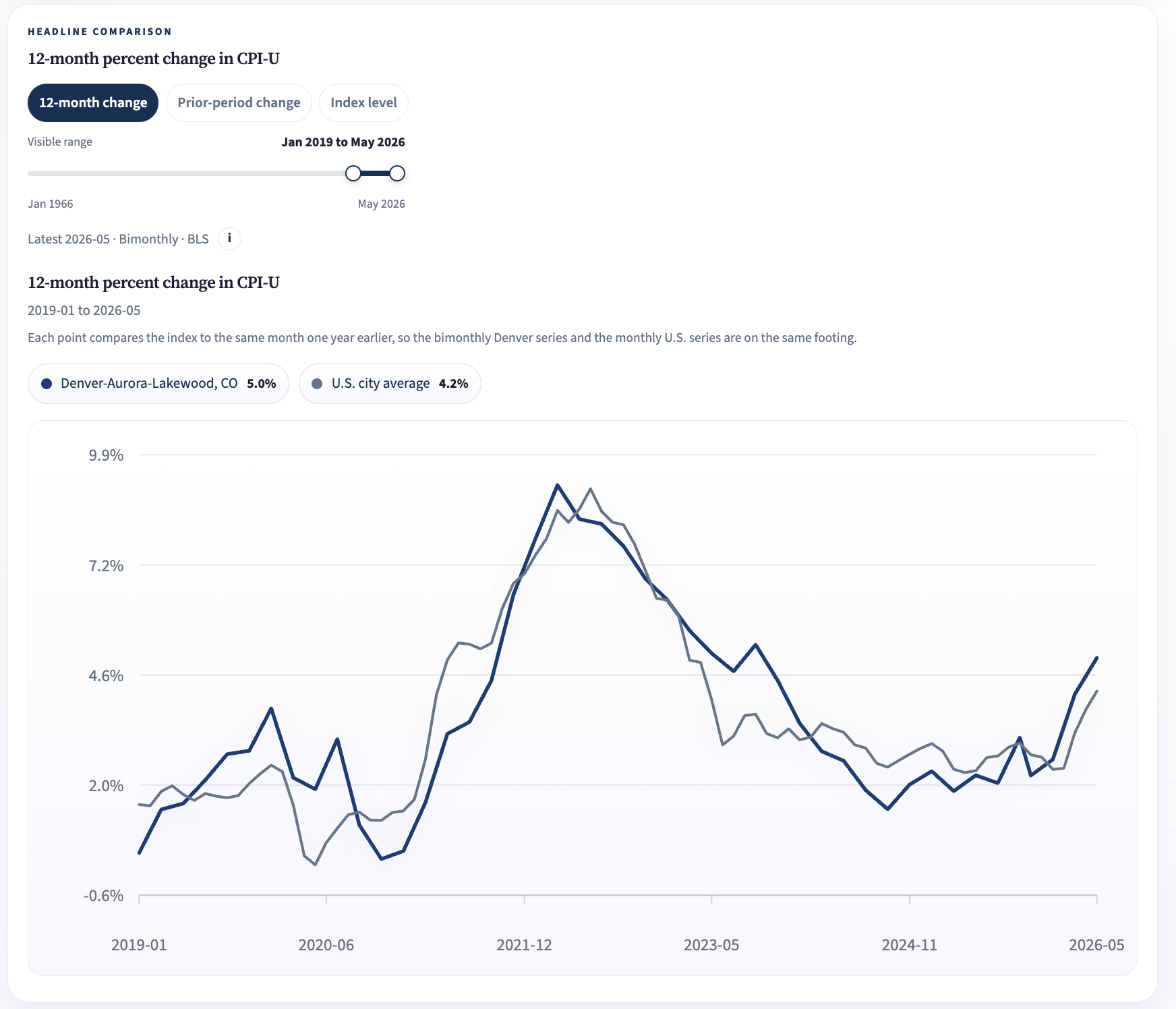
The 12-month change is the standard headline inflation measure, and right now it shows Denver-area prices up 5.0% over the year ending May 2026 compared to 4.2% for the U.S. city average.

One thing worth knowing when reading these charts is that the Denver MSA CPI is published every other month while the national series is monthly. That doesn’t matter much for the 12-month view, but in the prior-period view below, the Denver line shows two-month changes against one-month changes for the U.S., so the two lines are not directly comparable there (the chart notes this as well).

![](/images/posts/update-colorado-economic-indicators/img2.png)

![](/images/posts/update-colorado-economic-indicators/img3.png)

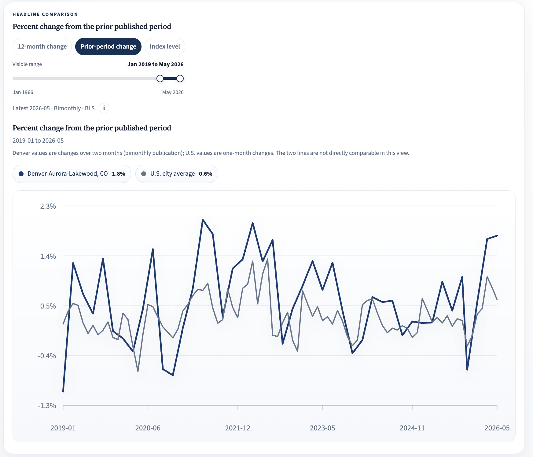
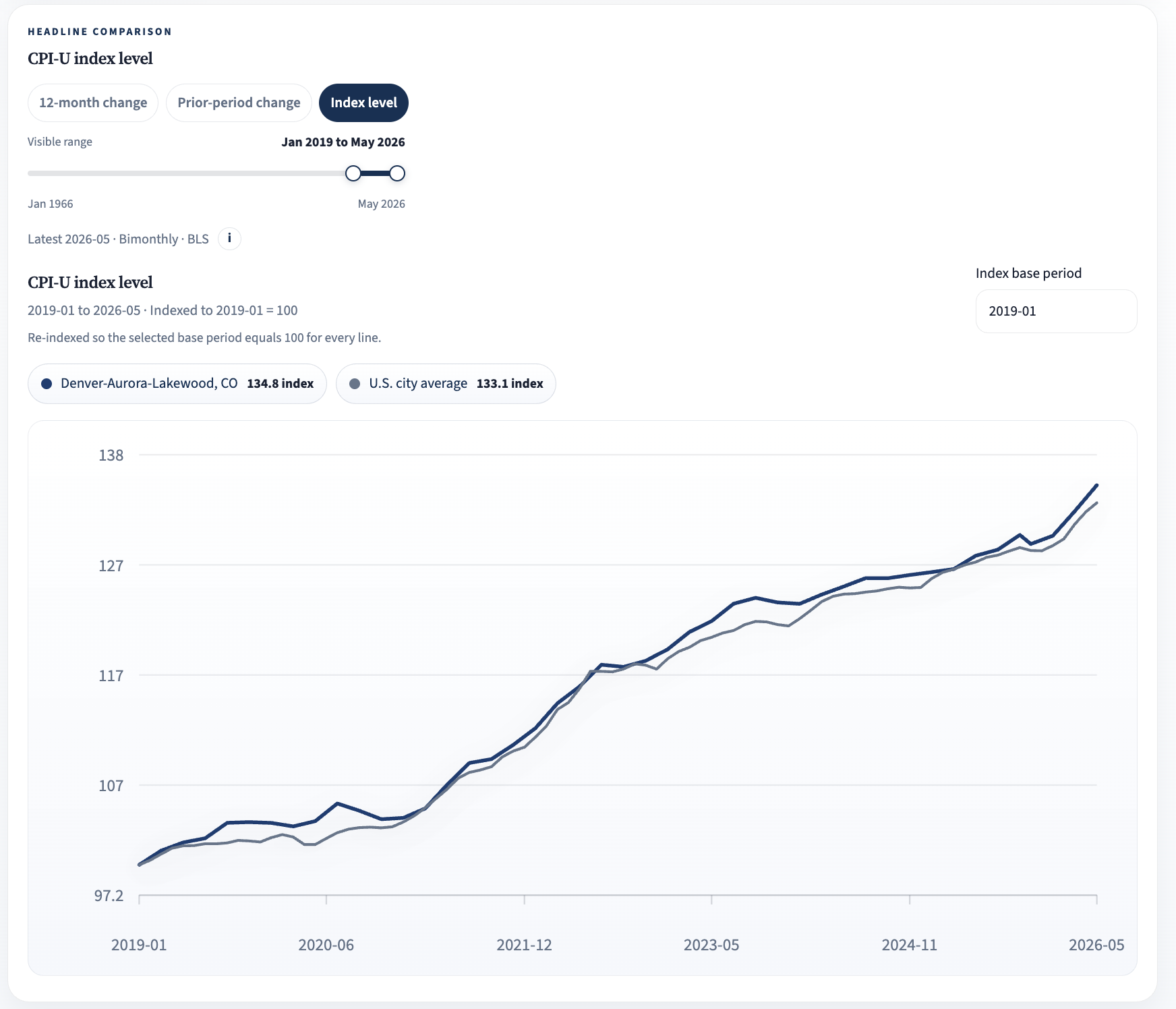
The index level view also lets you choose the base period, with every line re-indexed to equal 100 at whatever period you select. In the screenshot above, the base period is January 2019.

### Denver-Aurora-Lakewood MSA CPI Components Table

Below the chart is an interactive table where you can add or remove the published components of the Denver metro CPI, modeled on the BLS news-release table. Not every component is published for the Denver MSA, but the big ones are there including food, energy, gasoline, shelter, and all items less food and energy among a few others. Columns show the latest index value, the 12-month and prior-period changes for the Denver area, and the 12-month change for the U.S. city average. The table doesn’t allow comparisons across different time periods but gives a quick look at how the most recent price changes in the Denver area compare to the average around the country.

![](/images/posts/update-colorado-economic-indicators/img4.png)

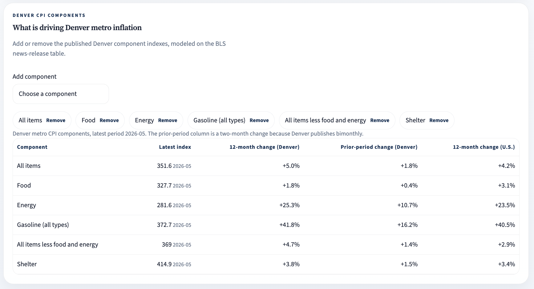
A standout in the screenshot above is gasoline. Gas prices in the Denver area are up nearly 42% over the year ending May 2026, compared to 40.5% nationally. The table also makes it easy to see what is driving the recent local numbers which most recently is energy, not shelter. Shelter prices in the Denver area are up a modest 3.8% over the same period while energy prices are up more than 25%.

As before, I added the inflation tab with the help of Claude Code.

---

# What’s Going on With Denver’s Restaurant Industry? (Part 2)

2026-05-18
Originally published on Substack: https://www.frontrangeeconomics.com/p/whats-going-on-with-denvers-restaurant-808

[Part 1](https://open.substack.com/pub/reillychandler/p/whats-going-on-with-denvers-restaurant?r=9i93a&utm_campaign=post-expanded-share&utm_medium=web) of this post on Denver’s restaurant industry looked at restaurant employment and establishments. I compared changes in both metrics relative to their 2019 levels using surrounding counties and a small group of “peer counties” to reach the following conclusions: 1) Denver full-service restaurants are in a clear slump, and 2) Denver limited-service restaurants are doing OK; employment and establishments are still above pre-pandemic levels. The first part of this conclusion confirms what [much](https://denverite.com/2025/02/27/denver-restaurants-closures-tipped-minimum-wage/) [local](https://coloradosun.com/2025/03/17/restaurants-closing-opening-data-denver/) [reporting](https://www.denverpost.com/2025/01/08/denver-restaurant-closures-numbers-since-pandemic/) and [other posts](https://open.substack.com/pub/matthewyglesias/p/denver-piece?r=9i93a&utm_campaign=post-expanded-share&utm_medium=web) on this subject have found, but I have not seen much of anything discussing the limited-service side of the problem. If you haven’t read that post already, check it out before getting into Part 2 here.

The conclusions from Part 1 are surprising for a couple reasons. First is that Denver appears to be facing a distinct problem among its full-service restaurants, suggesting that there are factors specific to Denver causing this. I wouldn’t go as far as to say this is unique to Denver. But across similar counties and other counties in the metro area, Denver stands out. Second is that the problem is mostly limited to full-service. In terms of both employment and establishments, limited-service restaurants are not struggling in the same way.

On the question of why this is happening, I want to be able to explain what it is about Denver but also differences across restaurant type to have a better understanding of why Denver’s full-service restaurants specifically are struggling so much. When I first started doing the background research and drafting for this follow-up post, I was going to cover a few different factors including labor costs, regulatory issues, and a bit on the demand side.

But as I continued working on this, the labor costs side of the story seemed to be the most compelling and will be the focus of what follows. Labor costs are among the chief concerns raised by operators as detailed in the *State of Denver Restaurants* report linked in the previous post. This complaint made sense to me as a real problem but some critics of the report have viewed this more as owners vs. workers and framed labor costs as a scapegoat for other issues. [Some critics of the report](https://www.denverpost.com/2026/04/16/denver-restaurants-oppose-tipped-minimum-wage-cut/) have even gone so far as to argue that there are simple conflict-of-interest reasons why the report focused on labor costs and the minimum wage. I believe the critics were too quick to dismiss labor costs as a major part of the story.

I will make the case that Denver’s minimum wage increases since 2020, particularly for the tipped minimum wage, can explain some of the full-service restaurant struggles. Then, I will propose a hypothesis related to this that can explain why limited-service restaurants in Denver are faring better. On the question of what can be done, I have more uncertainty. Given the evidence I show in this post, lowering Denver’s tipped minimum wage to the state level seems reasonable. What I am uncertain about is how much of an effect it would really have and how likely it is to happen as it seems like an unpopular idea.

I realize that this post is only looking at one among multiple causes of the decline in Denver’s restaurants and it would be silly to claim that there is a single cause that completely explains the decline. Too many things are happening at once that are impacting operating costs and the demand side for restaurants to really nail down what is happening in a single city. That doesn’t mean the minimum wage isn’t an important part of this story. For the reader who wants to look at evidence of other factors contributing to the general problem with Denver’s restaurants, I will link again to the *[State of Denver Restaurants](https://assets.simpleviewinc.com/simpleview/image/upload/v1/clients/denver/2025_State_of_Denver_Restaurants_Challenges_Facing_the_Sector_Final_a6d47ea4-e145-4b27-b90d-3447771f2df9.pdf)* report. That report isn’t the only source out there on this issue and was conducted on behalf of restaurant operators but does cover many different factors.

### Real Wages in Full-Service Restaurants: Denver vs. Comparison Counties

Before getting into the minimum wage, I want to show a couple of comparisons along the lines of what I did for Part 1 but now looking at real wages for full-service restaurant employees. I will be using QCEW data again to make these comparisons and the same two groups of comparison counties (neighboring counties and the peer counties group). From the QCEW data, I have nominal weekly wages for full-service restaurant employees in each county through Q3 2025. Then following the BEA’s method for implicit regional price deflators, wages are deflated using the product of the relevant Regional Price Parity (RPP) and the national PCE price index.<a href="#footnote-1" id="footnote-anchor-1" role="doc-noteref">1</a> I will use the same indexing strategy as before where the wages for each county are set to 100 in Q1 2019. Then, I can compare how wages have evolved since 2019 across these counties to see whether restaurant workers in Denver have experienced wage growth that stands out from comparison counties. I am also separating this from the minimum wage discussion that follows because wage gains that appear in this series are not representative of wage gains directly related to increases in the minimum wage. The minimum wage will have an effect but not for every restaurant employee captured in this data.

Because we are looking at total weekly wages divided by employee head count, the average weekly wage series for each county is capturing full-time employees, part-time employees, salaried employees, tipped employees, non-tipped employees, you get the idea. The point is, using this data alone, I don’t know what the composition of employees looks like and cannot make clear claims about how much of any wage increase is due to the minimum wage specifically. So even if wages are rising during the period of minimum wage increases in Denver, some of that might be due to the minimum wage increase, but some of it could also reflect a data artifact such as a shift toward full-time workers pushing up weekly wages or other factors unrelated to the minimum wage. But I still want to know how wages have evolved in Denver compared to other places to understand how distinct the labor costs problem actually is.

The first comparison shown in the chart below is between Denver county and neighboring counties which include Adams, Arapahoe, Boulder, Broomfield, Douglas, and Jefferson. Despite some declines during the height of the pandemic, all counties have experienced real wage growth relative to their levels at the start of 2019. But Denver leads the pack with around a 30% increase in wages relative to 2019. Keep in mind this is adjusted for inflation, so I am not simply capturing wages going up with prices in general. So at least among nearby counties, Denver stands out in the growth of its labor costs.

![](/images/posts/whats-going-on-with-denvers-restaurant-808/img1.png)

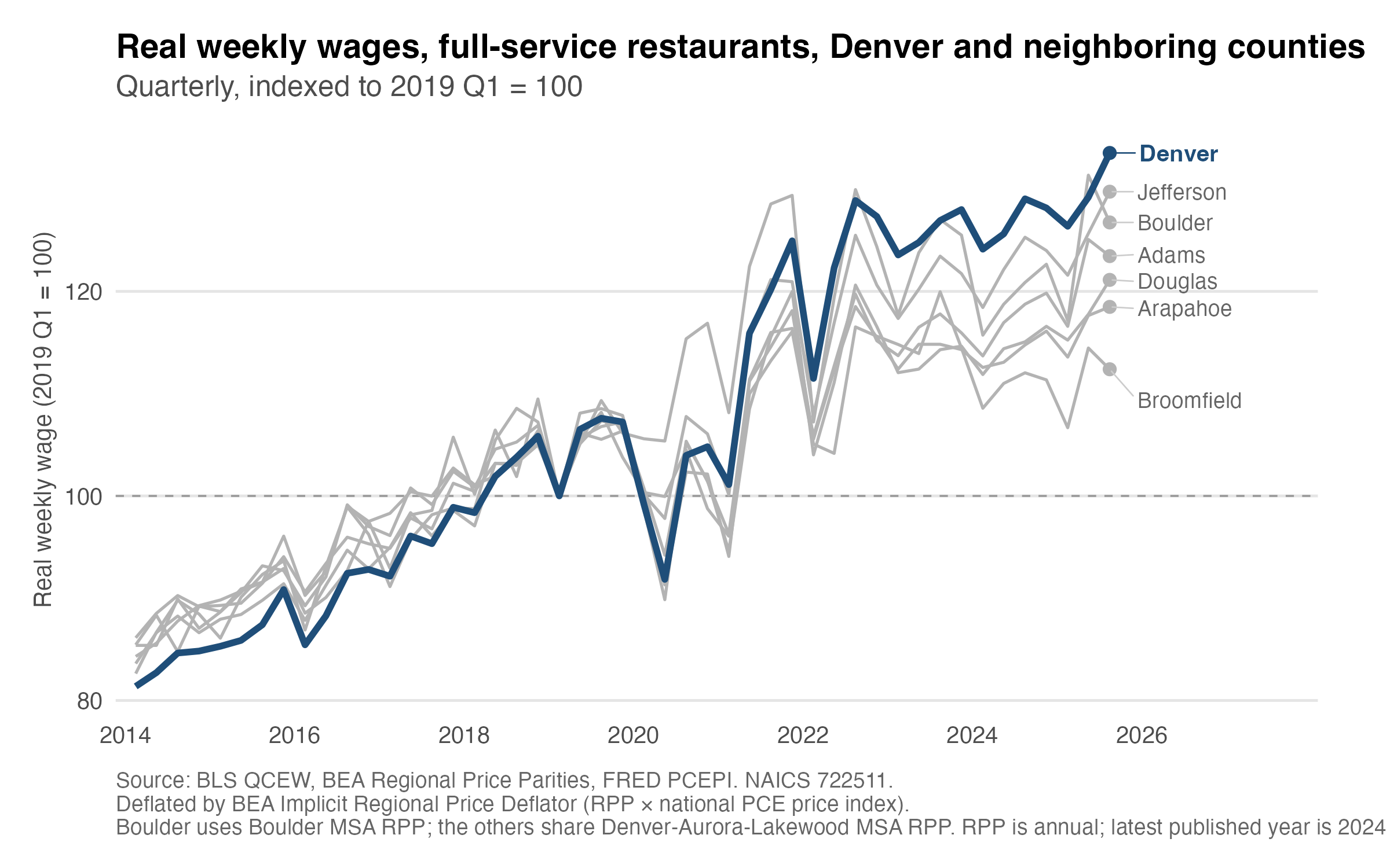
Now, let’s turn to comparing Denver to several peer counties including Davidson, Hennepin, Multnomah, Salt Lake, and Travis shown in the next chart. Note that labels correspond to the largest city in each county. The comparison is broadly similar to what was shown for neighboring counties. All counties have experienced growth in restaurant workers’ wages, but Denver leads the pack.

![](/images/posts/whats-going-on-with-denvers-restaurant-808/img2.png)

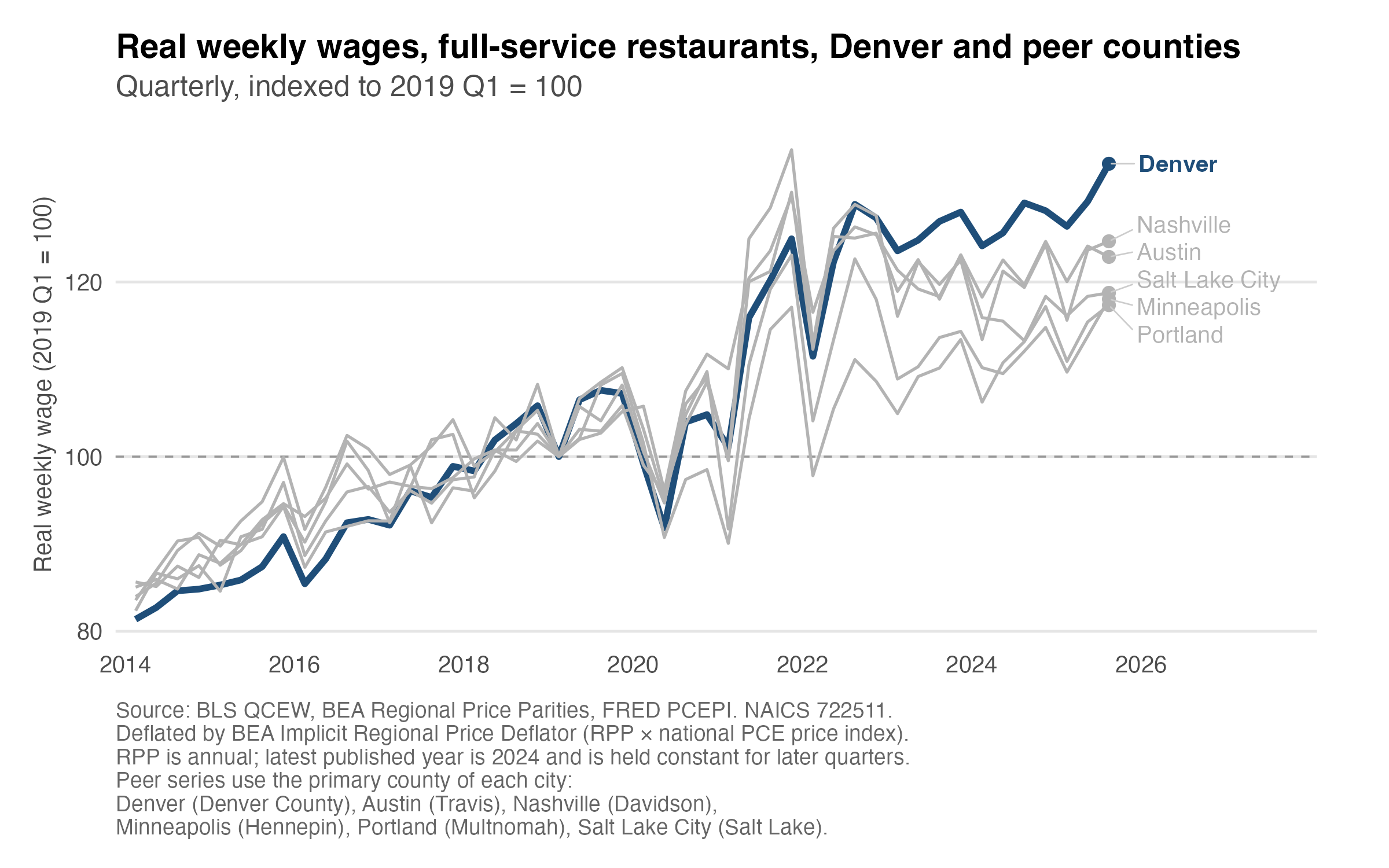
The comparisons paint a clear picture. Denver’s restaurant workers have achieved substantial wage growth since 2019 and at a level that stands out among its neighbors and some comparable counties. Next is to try to understand to what extent this can be attributed to the minimum wage.

### Denver’s Minimum Wage

Before assessing to what extent the rise in real wages is associated with the minimum wage, I want to briefly discuss the basic economic theory of minimum wage policy and the surrounding empirical literature on these effects.

First, let’s go over the effects of a minimum wage using the textbook model of a competitive labor market. For those unfamiliar with the supply and demand framework, this is a labor market where labor demand (the employer side of the market) is downward sloping, labor supply is upward sloping, and their intersection determines the going wage rate in that labor market. Employers will hire more labor hours the lower wages are (labor demand is downward sloping). Employees will work more labor hours the higher wages are (supply is upward sloping).

Absent any minimum wage policy, the market wage is determined by supply and demand. A minimum wage is a price floor in this market, and when it is set at a level above the wage determined by the intersection of labor demand and supply, we have a situation where employers are willing to hire fewer employee hours at this wage than workers are willing to work. The basic prediction of this model is that wages go up but the total number of hours hired in the market goes down.

The negative impact on employment is a directional prediction of the model. We’d need to know about the demand and supply curves and the minimum wage to get a better idea about the size of the impact on employment. However, this is also not the only model used to predict effects of the minimum wage. In a model where employers have market power, a minimum wage can increase employment and wages. How we decide which model’s predictions are correct is an empirical question.

Over the last few decades a sizable and increasingly sophisticated empirical literature in economics has found a range of effects of minimum wages in different contexts. In some cases, there appears to be no short-run effect on employment as in the famous Card-Krueger study. Others find positive effects and still others have found negative effects.

Arin Dube and Ben Zipperer created a database calculating what they call the own-wage-elasticity (OWE) which represents the percentage change in employment divided by the percentage change in minimum wage to arrive at a summary number of the impact of the minimum wage (see, [Dube’s post introducing the database](https://open.substack.com/pub/arindube/p/a-new-database-quantifying-the-minimum?r=9i93a&utm_campaign=post-expanded-share&utm_medium=post%20viewer)).<a href="#footnote-2" id="footnote-anchor-2" role="doc-noteref">2</a> Even when looking only at estimates compiled on studies from the U.S. for retail or restaurant workers, estimates range from large and negative to large and positive. But because each study is dealing with a different context and different increases in the minimum wage it is difficult to make any general empirical claims about the effects of the minimum wage. That does not mean, however, that no claims can be made about the empirical effects of the minimum wage. I’ll turn now to Denver’s local minimum wage which has been higher than the Colorado minimum wage since 2020.

Denver’s increases in the minimum wage since 2020 are not moderate especially when compared to increases in Colorado’s minimum wage (both tipped and non-tipped) as shown in the table below. And even if we restricted our attention to the labor market for restaurant employees, a reasonable assumption is that the market is competitive. So, as an initial prediction given these two facts, I would say the minimum wage likely causes some decrease in employment hours.

![](/images/posts/whats-going-on-with-denvers-restaurant-808/img3.png)

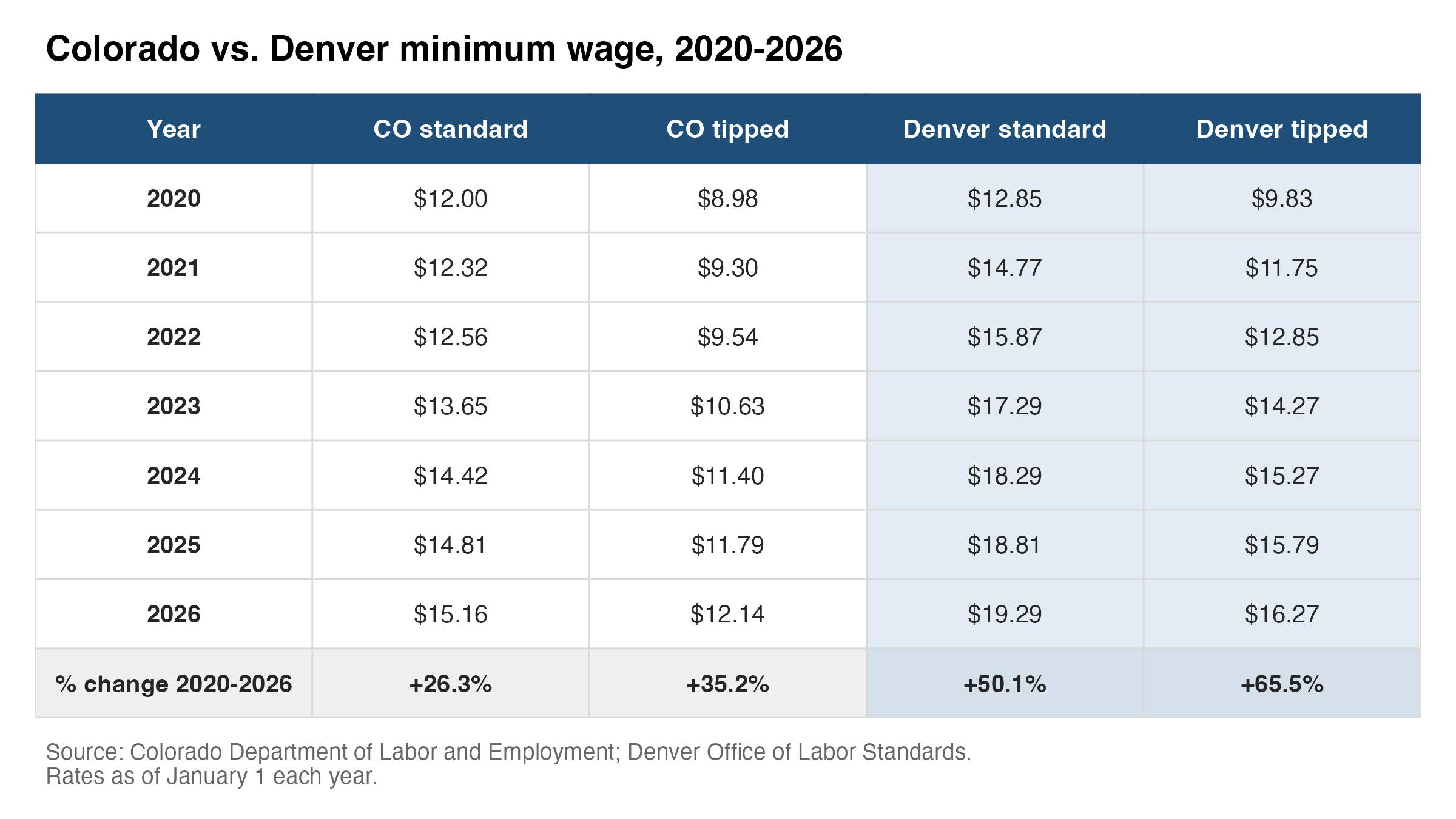
The minimum wage table above also shows a substantial difference in the growth of Denver’s tipped minimum wage relative to the city’s standard minimum wage (about a 15 percentage point difference). This on its own is going to cut against full-service restaurants more than it would for limited-service restaurants. Another relevant factor to consider here is how the employer side of the market responds to minimum wage increases over time. It has now been six years since Denver increased its minimum wage from the Colorado state level. And as [Brian Albrecht points out](https://open.substack.com/pub/pricetheory/p/how-can-price-theory-help-us-navigate?r=9i93a&utm_campaign=post-expanded-share&utm_medium=web), because demand is more elastic in the long run, we should expect the size of the employer response to minimum wage increases to grow over time. That is, the longer a minimum wage increase is in effect, the larger any downward adjustment in labor use among employers should be.

Put it this way, if you are a restaurant employer and the minimum wage increases it is unlikely that you are going to drastically cut employee hours the next shift or even during the quarter the increase occurs. But the longer that higher wage is in effect, the more you will adjust. Maybe you hire fewer seasonal workers or don’t rehire when an employee leaves. Maybe only the best of your staff get put on the schedule full-time going forward. This long-run adjustment framing will matter for how I think about the divergence between full-service and limited-service later in the post.

### Estimating Minimum Wage Effects in Denver

At this point, we know restaurant workers’ wages are high in Denver and have grown more than surrounding counties. The minimum wage has also increased substantially over the last several years. But how much of the increase in real wages is attributable to the increase in the minimum wage? To answer this question, I’ll refer to another recent [Substack post from Arin Dube](https://substack.com/@arindube/note/p-193623792?utm_source=notes-share-action&r=9i93a) which gave me the idea. In his post, Dube looks at several red states that adopted higher minimum wages and compares them to other states which stayed at the federal level as a natural experiment. The setup is straightforward, he looked at the differences in wages and employment between the states that did and did not adopt higher minimum wages before and after the adoption year. Then, the gap after the minimum wage increase gives some idea of wage changes that can be attributed to the minimum wage and the same for employment.

Luckily for me, Colorado presents a similar scenario where I can use this approach. With the exception of Boulder, Denver is the only nearby county to adopt a minimum wage above the state level in 2020. Denver is my treated county and the surrounding counties Adams, Arapahoe, Broomfield, Douglas, and Jefferson serve as the controls who stayed at the Colorado minimum wage. Denver and the surrounding counties also share a state policy environment that might affect restaurant operators’ labor decisions, such as Colorado’s FAMLI (covering things like maternity and paternity leave) and the state’s sick-leave policy. All of these counties also experience similar inflation. Any gap in wages and employment found between Denver and its neighbors should reflect factors specific to Denver, with the local minimum wage being the most obvious candidate.

Then, we can look at the evolution of restaurant wages and employment in Denver relative to the counties that did not adopt a local minimum wage and see what the gap looks like. To the extent that there is a positive gap in wages we can be more sure that wages are rising because of the minimum wage. Similarly, to the extent that there is a negative gap in employment, we can be more sure that the minimum wage is causing a decline in employment.

A brief note on what this is not. I am not presenting a rigorously specified empirical strategy to recover a causal estimate. There are some clear issues with this setup that would threaten clean identification. Edgewater, one of the cities that does have a higher than Colorado minimum wage, is in Jefferson county but is being treated as a control. That poses the threat of downward bias on the estimated growth in wages due to the minimum wage in Denver. Also, the state minimum wage has not been fixed since 2020; it has just grown more slowly than Denver’s. The “control” counties are therefore not genuine controls. They did have increases in the minimum wage, just smaller increases than took place in Denver. Because of this, we should expect bias toward zero for any wage and employment effects estimated. However, this approach should be more informative than the naive comparisons earlier in the post in part because if there are substantial increases in wages and substantial decreases in employment relative to surrounding counties, we should expect that those would be more pronounced using a cleaner control set.

The chart below shows the side-by-side results for this approach on full-service restaurant wages and employment. Both are set to 0 in Q1 2019, and what we see for wages is that by late 2025, real wages for full-service restaurant workers in Denver had grown about 12 percentage points more than wages in surrounding counties relative to their 2019 levels. This gap is consistent with Denver’s minimum wage increases driving a meaningful share of Denver’s recent wage growth, though how much exactly is not clear. The right-hand panel shows substantial declines in restaurant employment at the same time wages are rising. By late 2025, full-service restaurant employment in Denver was more than 10 percentage points lower than employment in surrounding counties relative to 2019.

Again, I won’t pretend these are causal estimates. We have some evidence that Denver’s restaurant workers’ wages increased as the minimum wage increased and more so than neighboring counties that stayed on the lower state minimum wage. We also have evidence that restaurant employment declined over the same period and substantially more than in neighboring counties. This pushes me closer to believing that the minimum wage increases in Denver can explain some of the decline in the restaurant industry.

![](/images/posts/whats-going-on-with-denvers-restaurant-808/img4.png)

From the perspective of restaurant owners, this means they could face a few dollars an hour difference in labor costs per employee when determining to open in, say, the city of Wheat Ridge in Jefferson County or in Denver. That doesn’t imply that most operators are going to choose Wheat Ridge just to save on labor costs. Foot traffic differs across these locations and the hit to the consumer base may be more than enough to offset labor cost savings, but this will matter on the margin. Operators have a clear cost incentive to open restaurants in surrounding counties and opt out of Denver.

### What About Limited-Service Restaurants?

The remaining piece of the puzzle though is why limited-service restaurants are not doing as poorly. Higher labor costs can explain why Denver restaurants under-perform those in surrounding counties, but not the full-service vs. limited-service divergence. Now, I will get back to the long-run elasticity point to present a hypothesis. More adjustment on the labor-demand side doesn’t just mean that full-service restaurants use less labor and that some eventually exit because they can’t make it. It might also mean that additional adjustments are being made to have a more permanent reduction in labor use. And one way to do this is to adjust the business model of the restaurant before it opens.

I’ll start with the premise that full-service restaurants tend to be more labor-intensive businesses than limited-service restaurants. A full-service restaurant will have to hire wait staff, hosts, cooks, people to clear tables, dishwashers, etc. Maybe in the face of higher labor costs, operators begin to combine employee tasks. Wait staff handles clearing tables, and there are no busboys. There is no host position and wait staff handles customers as they come in. Cooks double as dishwashers. But even with some expansion of job duties to cut down on staff, we should expect limited-service restaurants to have fewer employees on average.

Limited-service restaurants still have cooks and people to handle orders at the cash register but there is no wait staff, no need for hosts, and combining tasks is relatively easier. Cashiers can collect trays and clear off tables when there are lulls in the line (customers might even handle some chunk of this). Shifts can overlap, so cashiers handle other tasks toward the end of their shift and the employee coming in takes over at the register. Luckily, the QCEW data I have been using across these two posts does allow me to at least present a proxy for the sort of labor intensity I am describing here.

The proxy measure I have in mind is simply average employees per establishment by restaurant type. That is, the employee headcount divided by the number of establishments for both full-service and limited-service restaurants. Admittedly, this measure is not perfect. Restaurants of both types will vary in how many employees they have, and headcount might overstate labor intensity. For example, a restaurant with more part-time employees may appear more labor-intensive than one with fewer (but more full-time) employees putting in the same total hours. But as shown in the chart below, there is a clear and persistent gap in the average number of employees per restaurant across types.

![](/images/posts/whats-going-on-with-denvers-restaurant-808/img5.png)

Prior to the pandemic, this gap was much larger. Full-service restaurants had around 9 more employees per restaurant than limited-service restaurants on average. Since the pandemic, the gap remains but has shrunk. Full-service restaurants now have something closer to 5 more employees per restaurant than limited-service restaurants. The gap shrinking is consistent with the idea that full-service restaurants have had to figure out how to combine tasks or adjust to operating with fewer employees. However, it is also consistent with larger restaurants exiting and leaving behind more full-service restaurants that hire fewer employees, even without any task combination. The persistent gap across restaurant types *is* consistent with the starting premise that operating a full-service restaurant tends to be more labor-intensive than operating a limited-service one, even if task adjustments or some other factor have occurred to shrink the gap. And if full-service is more labor-intensive than limited-service, then a minimum wage increase raises full-service operating costs by more than limited-service costs in percentage terms.

With this difference in labor intensity across restaurant types in mind, let’s imagine someone looking to open a restaurant. Our restaurateur plans to open a full-service restaurant and she starts thinking about hiring. She will need to hire wait staff, cooks, a manager, and maybe hosts. Each of these employees must be paid at least the minimum wage or the tipped minimum wage depending on their role. After doing some back-of-the-envelope calculations, she sees how much revenue she’d have to bring in to break even with these costs and realizes it just won’t work. The restaurant would have to be a massive success just to cover costs.

At this point, our new restaurant owner may just give up but that is not the only option. She could tweak her plan a bit and open as a limited-service restaurant. Why might this be a solution? The restaurant with counter-service can be a way to permanently lower labor costs. The first cut would be to the wait staff. A few people to staff the cash registers, who may also perform other tasks, means fewer people adding to the total wage bill. She still needs cooks and a manager, but overall the total number of employees and working hours can easily be slashed before the restaurant even opens. And in this scenario she still gets to open a version of her restaurant.

The more labor costs rise and the more permanent these changes are, the more likely we should expect this decision to be made. That is one channel through which the long-run adjustment to the minimum wage increase can take place.

The difficulty with this hypothesis is that it’s not clear how or where it would show up in the data. It is unlikely that there are many full-service restaurants making the switch to limited-service. But if that were happening, I am not aware of a dataset that would allow me to see something like reclassification from full- to limited-service. Similarly, I am not aware of any dataset at the county level with detailed industry classification for gross flows of establishments. And what I have in mind is at the stage of planning or getting ready to open a new restaurant, some operators are opting to go with the limited-service model. This isn’t something that would be captured in any data that I am aware of.

The best I can do with the data I have is to do the same “natural experiment” comparison done for full-service this time for limited-service and see the wage and employment gaps for limited service in Denver compared to surrounding counties that adhere to the state minimum wage. This evidence will not tell me whether more operators are choosing limited-service. What it does do is allow me to see whether wages for limited-service workers have risen relative to surrounding counties more or less than was the case for full-service restaurants.

If the relative wage increases are less, then limited-service restaurants are not only less labor-intensive but also less costly to operate in Denver relative to surrounding counties, making the monetary incentive for adjustment clearer. The minimum wage might also produce similar increases in wages for limited-service employees as it did for full-service employees. Even in this case, however, there is still a difference in cost hit. As discussed above, there is a persistent gap in labor intensity across restaurant types.

If my hypothesis is correct, I would also expect any declines in employment in the limited-service sector to be weaker than those found for full-service. But if both wage gains and employment declines are close to the same for limited-service, it’s unlikely this entry-adjustment idea is correct. At best, this is evidence of the shift in incentives between operating a full-service and a limited-service restaurant, not the outcomes predicted by my hypothesis.

The chart below shows the side-by-side comparison of wages and employment for limited-service restaurants in Denver relative to the neighboring counties. The left panel suggests that wages for limited-service restaurant workers have risen similarly to those in full-service, 10 percentage points for limited-service compared to 12 percentage points for full-service. These numbers are close enough to suggest that the minimum wage has likely affected wages in both sectors equally. The changes in employment are not the same, however. Although in the most recent periods there is a negative employment gap, it is much smaller than the one for full-service restaurants. Limited-service restaurant employment is around 4 percentage points lower in Denver than in surrounding counties as of late 2025. The same figure for full-service employment was more than 10 percentage points lower.

![](/images/posts/whats-going-on-with-denvers-restaurant-808/img6.png)

The wage finding shows the minimum wage affected per-worker pay in full-service and limited-service about equally. But because full-service restaurants employ more workers per establishment (even as employment has declined for full-service), the total cost per restaurant is larger for full-service. The cost advantage of limited-service has only widened as Denver’s minimum wage has risen, consistent with the hypothesis that the divergence across restaurant sectors can also be partly explained by the minimum wage. If someone is looking to open a restaurant in Denver, the incentives are pointing toward a limited-service business model.

### What to Do?

Where does this leave us? Even without a clean causal estimate, the evidence is consistent with Denver’s minimum wage increases lifting restaurant wages above what surrounding counties saw and weighing on restaurant employment. There is also evidence that this is not affecting limited-service restaurants to the same extent. Together, the evidence suggests that both the distinct problem of Denver’s restaurants and the divergence across sectors of the restaurant industry can be partly explained by Denver’s minimum wage.

There is a limit to what this means for policy though. Even if I think that the broader market for low-wage labor in Denver is competitive and the recent increases in the minimum wage have been large enough to cause employment declines more generally, the evidence shown here is strictly on restaurants and even within that sector there is variation. I wouldn’t confidently say that Denver should revert the minimum wage to the state level because the story may not be the same in different areas.

But the Colorado state legislature passed a law last year which would allow cities like Denver to bring their tipped minimum wage closer to the state level. [Governor Polis explicitly](https://www.westword.com/food-drink/colorado-governor-signs-controversial-tipped-wages-bill-into-law-24738279/) called on Denver and other cities in Colorado with higher minimum wages to address the tip credit when this law passed. Given what I have shown here this is a reasonable policy. Denver’s tipped minimum wage being lowered to the state level will probably provide some relief to full-service restaurants. And if we wanted restaurants to be doing better, the seemingly obvious response would be to do this. The problem, however, is that this seems politically unpopular. As far as I know, there hasn’t been any formal discussion of this issue in the Denver City Council yet but advocacy groups and over 50 restaurants have already [urged the city](https://www.denverpost.com/2026/04/16/denver-restaurants-oppose-tipped-minimum-wage-cut/) not to reduce the tipped minimum wage. Maybe there is some support and this will happen but I’m not optimistic.

Despite the seeming unpopularity, I want to make the case that lowering Denver’s tipped minimum wage is limited in scope and worth taking a chance on. Tipped workers are concentrated in the restaurant industry and lowering the tipped minimum wage limits the scope of impact. It also doesn’t necessarily lead to an outcome where restaurant workers, especially those who are typically tipped, go through a decline in wages. The tip credit already operates so that employers must make up the difference if a tipped worker’s base wage plus tips falls below the non-tipped minimum wage. So, the minimum wage floor is still there. What changes is who pays for the floor, employers or customers. Restaurant operators can also choose to pool tips or eliminate tipping. Some will do this and can pay their wait staff the higher non-tipped minimum wage. Other operators will choose the lower tipped minimum wage and allow tips. Workers can then figure out which is the better deal, and job switching will occur over time.

If Denver does revert to the Colorado tipped minimum wage, I would not expect a rapid recovery in full-service restaurants. The downward adjustment took time and so would any recovery. Maybe this new equilibrium with fewer full-service restaurants is fine, but I wouldn’t mind seeing more restaurants popping up. Denver is an underrated food city, and making it easier for operators to experiment and provide consumers with more options would be great to see.

<a href="#footnote-anchor-1" id="footnote-1" role="doc-backlink" aria-label="Back to reference 1">1</a>

There are a couple limitations to using the RPP values here to adjust for more local infaltion than the national PCE price index alone: 1) RPPs are only available annually, I am using the same value for every quarter in a given year, and 2) They are constructed at the MSA-level not the county level which the wage data is at.

<a href="#footnote-anchor-2" id="footnote-2" role="doc-backlink" aria-label="Back to reference 2">2</a>

Arin Dube’s post explaining OWE in more detail is linked above but for quick reference: When OWE is less than or equal to -1, an increase in the minimum wage is more than offset by the decrease in employment (low-wage workers are generally worse off). When OWE is greater than -1 (even if still negative), low-wage workers are better off. And here is a link to [the database](https://economic.github.io/owe/).

---

# Who Needs a License to Work in Colorado?

2026-09-28
Originally published on Substack: https://www.frontrangeeconomics.com/p/who-needs-a-license-to-work-in-colorado

In a couple of posts here at Front Range Economics, I have been critical of some labor market regulations such as Denver’s minimum wage (see [part 2 of my Denver restaurants post](https://www.frontrangeeconomics.com/p/whats-going-on-with-denvers-restaurant-808?lli=1)) and Colorado’s childcare regulations (see my [childcare costs post](https://www.frontrangeeconomics.com/p/the-cost-of-child-care-in-colorado?lli=1)). For this post, I’ll highlight an area of labor market regulation where Colorado is much less restrictive compared to the rest of the country and make the case that this is a good thing.

To compare Colorado to the rest of the country I will rely on the 2026 edition of the [Archbridge Institute’s State Occupational Licensing Index](https://www.archbridgeinstitute.org/state-occupational-licensing-index/). In this index, Colorado has the 5th fewest occupational barriers and is ranked the least restrictive in the Mountain West region. Colorado restricts among the fewest occupations in the country and has a universal recognition law, enacted in 2020 and revised in 2022, that allows individuals from many occupations licensed in other states to move here, transfer their license, and get to work.

Not everyone views Colorado’s [lax occupational licensing as good policy](https://krdo.com/news/2024/02/23/families-push-to-change-lax-funeral-home-laws-after-numerous-tragedies-across-the-state/). For instance, in response to the [Return to Nature funeral home case](https://www.nbcnews.com/news/us-news/ex-owner-colorado-funeral-home-decomposing-bodies-found-sentenced-30-y-rcna342025), politicians and the public were quick to blame the lack of licensing for creating an environment where this could occur. The state will start licensing some funeral occupations in 2027. I see why the public and the state responded with calls for licensing in this industry, but it’s [not clear licensing would have stopped these abuses](https://marginalrevolution.com/marginalrevolution/2026/06/colorados-funeral-mistake.html), and [some reporting suggests](https://apnews.com/article/colorado-funeral-home-bodies-found-investigation-ee1089fab926042fda05fe5fa79ec7ce) this was a failure to regularly inspect funeral homes.

Outside the specific case of occupations in the funeral industry, [recent research on occupational licensing has shown](https://static1.squarespace.com/static/5efd3aa2efdd52166bd4f64b/t/6877b43407e3d73b8a271ad2/1752675381224/occupational-licensing.pdf) that there can be benefits to limiting licensing, especially when the case for consumer protection is weak. And Colorado seems to have most of its licenses concentrated in occupations with stronger consumer protection justifications (think doctors and lawyers), suggesting the state’s licensing burden is small relative to more restrictive states such as Oregon. But Colorado is not some occupational wild west.

The rest of this post will elaborate on the case for limiting occupational licenses, present the Archbridge index data for Colorado, and then illustrate one of the limitations of the index when it comes to comparing stringency in licensing across occupations.

### Is less occupational licensing desirable?

Occupational licenses act as a costly screen to enter a profession using some combination of minimum requirements. These requirements might include a certain number of educational hours to become a cosmetologist. Or a degree and an exam before receiving a license, as in nursing or law. Other licenses are pretty minimal in their requirements. There might just be an online test and a small fee.

One argument in favor of licensing is that these requirements ensure a minimum level of competency in an occupation and avoid the imposition of search costs associated with figuring out who the decent cosmetologists and nurses are, to the benefit of the consumer. If the state sets standards, all consumers and employers can be reasonably sure the barber or lawyer they’re hiring is not a total fraud. [Recent research from economist Nicholas Carollo and co-authors](https://static1.squarespace.com/static/5efd3aa2efdd52166bd4f64b/t/69f4d379c4811546ab5660d3/1777652601803/origins-and-evolution.pdf) provides some theoretical and empirical support for this argument. They look at the history of occupational licensing in the U.S. and show that occupations are more likely to be licensed the more relevant consumer protection concerns are.

But that doesn’t mean licensing is only ever about consumer protection. Carollo and his co-authors also show that members of some occupations, represented by professional associations, seek licensing laws to protect wages in their industry. They may make public-interest arguments, but they’re after a wage premium. And even if a license or a barrier raised the average quality of service for a profession, that is not an obvious positive for consumers. Consumers who cannot afford the level of quality at the licensed level are priced out of the market. A reduction in entry costs may make it possible for lower quality entrants to offer services at a lower price. Depending on what occupation we are talking about, it may be better to have access to a lower quality version of a service than none at all. Where this is true, it is a point in favor of weakening licensing restrictions.

For something like a doctor or a lawyer, a stronger case can be made for the state stepping in and saying we aren’t going to let these people sell medical or legal services if they can’t meet this standard. Many occupations that are licensed, however, have much weaker consumer protection justifications.

Think about cosmetologists or barbers, occupations requiring many hours of education to obtain a license in most states. Sure, we want our barbers and cosmetologists to be competent, but there are strong market incentives for them to be competent. A barber who consistently gives terrible haircuts or uses dirty tools won’t keep a job for long whether hired by a chain like Great Clips or running their own small business. In these cases, licensing raises the cost of entry, which likely brings a wage premium and higher prices for the service.

Maybe you think the consumer protection case for barbers and cosmetologists is stronger than I’m making it out to be. Fine. But look at the occupations licensed in many states, and it is not hard to see how weak the consumer protection justification is for many of them.

Although I do think there are [feasible options for something like private certification](https://www.wsj.com/arts-culture/books/the-licensing-racket-review-theres-a-board-for-that-3da68d0a?st=BaiWwK&reflink=desktopwebshare_permalink) to replace state occupational licensing, I don’t see occupational licensing as an illegitimate function of the state. I’m not making an argument for the abolition of all occupational licensing.

I’ll cite [another recent paper from Nicholas Carollo](https://static1.squarespace.com/static/5efd3aa2efdd52166bd4f64b/t/6877b43407e3d73b8a271ad2/1752675381224/occupational-licensing.pdf) to further support the point that while some occupational licensing can be beneficial, this is not true for all occupations. He finds that licensing is generally associated with persistent wage premiums and rising employment, but that for occupations where licensing has a weaker consumer protection justification (he uses the example of florists), employment effects are more likely to be negative. So, in occupations where the consumer protection justification is weak, we may end up with higher prices *and* less competition. That’s a stronger case for not licensing those occupations.

Now on to the index data.

### The Archbridge Institute State Occupational Licensing Index 2026

The Archbridge Institute has published its occupational licensing index since 2023, and I use the 2026 edition here. The [full report](https://www.archbridgeinstitute.org/state-occupational-licensing-index/) describes the method in detail, and Edward Timmons (VP of Policy at Archbridge and one of the authors of the report) [wrote about the release](https://edwardjtimmons.substack.com/p/2026-state-occupational-licensing?r=9i93a&utm_campaign=post-expanded-share&utm_medium=post%20viewer) on his Substack. I’ll briefly go over its methodology so the charts I show are clear.

The index covers 246 occupations and indicates whether each occupation is explicitly licensed or faces a barrier in all 50 states and Washington, D.C. From the Archbridge report on the distinction between a barrier and a license:

> In our index, we define a barrier to mean that the tasks associated with an occupational title are restricted by an occupational license. A license is an explicit license for that occupational title. For the state of Alabama, “acupuncturist” has a barrier, a physician license, but no explicit “acupuncturist” license. If the SOLI index were calculated with physicians and acupuncturists only, Alabama would have a barriers count of two and a licenses count of one.

In other words, every license is a barrier but not every barrier is a license.

Using this data, each state is assigned a barrier score and a license score based on the report’s index formulas. These scores capture the breadth of barriers and licenses relative to their respective ranges across states. Finally, the report ranks states from the most restrictive (#1) to the least restrictive (#51) by their barrier score, with ties broken by license score.

In addition to the ranking based on barriers and licenses, Archbridge categorizes states by their universal recognition status. Many states have no universal recognition laws on the books, so anyone who moves there must get a new license, even if they already hold one from another state. But 28 states have some form of universal recognition law. Archbridge categorizes these states by a “medal” status of gold, silver, or bronze. A gold medal state has no “substantially similar” clause *and* no residency requirement. A silver medal state has a residency requirement but no substantially similar clause. A bronze medal state has a substantially similar clause and may also require residency.

Let’s look at where Colorado lands in this index.

### Where Colorado lands

Colorado’s overall ranking in the index is at the 5th least occupational licensing (47th out of 51). Only New York, Indiana, Missouri, and Kansas have fewer barriers than Colorado. There are 132 distinct barriers for occupations in Colorado (5th fewest) and 102 occupations are explicitly licensed (2nd fewest), while the national averages are 156 for barriers and 122.6 for licenses. The charts below show these numbers for Colorado and all other states ranked from most to least. If you want to work in Colorado, there are fewer barriers in your way to get going in an occupation than in many states around the country.

<img src="/images/posts/who-needs-a-license-to-work-in-colorado/img1.jpeg" alt="" width="1456" height="1257">

We can also compare Colorado to other states in the Mountain West. In the region, Colorado has the fewest barriers, one fewer than Wyoming, and the 2nd fewest licensed occupations, two more than Wyoming.

<img src="/images/posts/who-needs-a-license-to-work-in-colorado/img2.jpeg" alt="" width="1456" height="699">

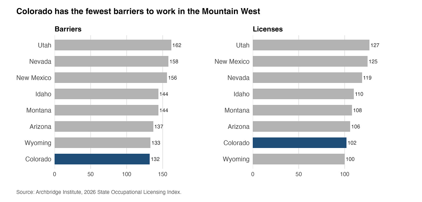Colorado, like every other state, licenses occupations such as attorneys, nurses, dentists, pharmacists, and public school teachers. But Colorado’s most uniquely licensed occupation is psychiatric technician, for which only 4 states require a license. According to the BLS description, a psychiatric technician is someone who provides “[care for people who have mental conditions or developmental disabilities](https://www.bls.gov/ooh/healthcare/psychiatric-technicians-and-aides.htm)” and [OEWS data for 2025](https://data.bls.gov/oesmap/) shows there are fewer than 2,000 people working in this occupation in Colorado.

For another look outside the index itself but using Archbridge’s data, we can see the occupations that face no barrier in Colorado but would in most other states. The chart below shows 10 occupations where this is true.

<img src="/images/posts/who-needs-a-license-to-work-in-colorado/img3.jpeg" alt="" width="1456" height="837">

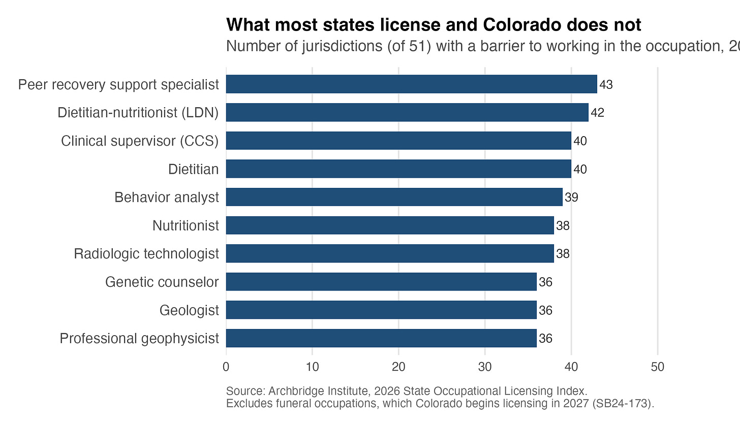If you want to work in any of the occupations on this list, Colorado is the place to be. At the top is peer recovery support specialist, which has a barrier in 43 states. These are people in recovery from addiction or mental health challenges who provide support for others going through the same. There are also three related occupations (dietitians, dietitian-nutritionists, and nutritionists) that face barriers in most states. Here you might be able to make a strong public interest case for licensing, but there are also many different approaches to diet and nutrition that a licensing program, in an effort to standardize, might restrict. We also have geologists on the list. Who knew Randy Marsh was unlicensed all this time?

<img src="/images/posts/who-needs-a-license-to-work-in-colorado/img4.jpeg" alt="" width="1456" height="819">

On universal recognition, Colorado earns a gold medal thanks to its 2020 universal recognition law that was later revised in 2022. The law created Colorado’s license portability program intended to make it easier for people to move here with an out-of-state occupational license and start working in their occupations. However, two caveats apply to Colorado’s medal status here.

First, the state’s universal recognition law has exceptions for several occupations, including electricians, plumbers, and outfitters. Second, the 2022 revision narrowed the law’s “substantially similar” clause but did not remove all substantially similar language. It allows individuals licensed in another state for at least a year, with a substantially similar scope of practice, to transfer their license. Given there are only three medal categories, it seems fair that the authors of the report placed Colorado in gold. I raise these two points only for additional clarity.

The Archbridge index gives a great overview of where Colorado stands relative to the rest of the country, but no index is perfect. There are some limitations to how the data can be used.

### Stringency across a few occupations

I’ll focus on just one limitation in this data, which is that it *only* looks at the breadth of occupational regulation. Barriers and licenses are counted up and used to make the relative comparisons across states. This makes the comparisons straightforward but won’t tell us anything about how difficult it is to obtain different licenses. If we look at what it takes to get a license in a couple of occupations in Colorado, we’ll get some sense of how much stringency varies. In some cases, the restrictions present barriers to entry that make it much harder for people to work in a given occupation, while others aren’t much more than an application and a small fee.

Take two examples on opposite ends of the stringency spectrum. [Requirements to become a licensed pharmacist in Colorado](https://drive.google.com/file/d/14jIuS_Uo5XlCBrNcKOwCJEtKTwijfDPA/view) include a doctor of pharmacy degree, 1,500 intern hours, passing license and jurisprudence exams, continuing education hours, and exam fees. I’d say this occupation falls into the more stringent category when comparing occupations and likely does in most states. At the other end of the spectrum, we have an occupation like pyrotechnic operator. This is probably no surprise, but it is a lot easier to obtain a pyrotechnic operator license in Colorado than a pharmacist license. [The requirements here](https://dfpc.colorado.gov/sections/professional-qualifications-and-training/certification/fireworks-certification) are limited to a background check, prior experience, proof of safety training, passing a general fireworks knowledge exam, and a \$50 fee.

The point of these two examples is simply to illustrate how different licensing requirements can be. The extent to which Colorado has less of a licensing burden than other states is only partially explained by the breadth of licensing. We would need a deeper look at requirements across all licensed occupations within Colorado and across other states as well as how many workers these rules affect to get a full picture of the burden. Looking at breadth is a good start, but only part of the story.

### Conclusion

So who needs a license to work in Colorado? I won’t pretend I can put an exact number on it because of the issues discussed above. But I can say that relative to most other states, there are many more occupations where legal barriers to entry don’t exist in Colorado. Even if you are someone who is generally in favor of regulation, you might also appreciate that Colorado does license the occupations where you’d worry the most about the lack of government intervention, including physicians, dentists, lawyers, nurses, teachers, and so on. What the state does not do (in most cases) is create barriers to occupations like auctioneers or home inspectors, where it is much harder to make the public interest case.

---

# What's Going on with Denver's Restaurant Industry? (Part 1)

2026-05-01
Originally published on Substack: https://www.frontrangeeconomics.com/p/whats-going-on-with-denvers-restaurant

I moved to Denver after graduate school, and before my wife and I made the move people would ask us about plans to get into skiing or hiking, typical Colorado stuff. I was definitely excited about doing more outdoor activities, but was most excited about exploring the food options in a new city. My wife and I love trying new places and after living in the D.C. area for five years, we were interested to see what Denver had to offer. It wasn’t long before we found a wide variety of restaurants in and around Denver with awesome food. I even started putting a note in my syllabus encouraging students to email me their favorite restaurants in the area for a little extra credit so we always had new places to try.

Sadly though, we arrived in Denver in what appears to be a period of struggle for the city’s restaurant industry. In the few years we have been here, many places we enjoyed eating at have closed, some after not even a year of being open. One example is [EatYa Pizza](https://www.westword.com/food-drink/16th-street-mall-restaurant-eatya-pizza-closing-23478125/), which used to be on the 16th Street Mall and was only open for 9 months. EatYa was excellent. Roman style pizza by the slice with unique toppings at a decent price. I could walk over there from my office for lunch to grab a couple slices and have a better lunch than the sandwich I usually bring from home. It was somewhere I took people when they came into town to visit or just to grab dinner to-go and eat at home.

EatYa was not a one-off closure it seemed. Even just along the 16th Street Mall since living here other restaurants have come and gone including a great Asian spot (YumCha). Local reporting over the last few years has brought up [again](https://www.axios.com/local/denver/2025/01/27/colorado-restaurant-industry-closures) and [again](https://www.denver7.com/news/360/why-are-so-many-denver-restaurants-going-belly-up-or-moving-out-of-the-city) and [again](https://www.westword.com/food-drink/biggest-denver-restaurant-closings-of-2025-40821928/) that both consumers and operators are frustrated and feeling like the restaurant industry has gotten more difficult. These problems have become severe enough that Denver Economic Development & Opportunity, Visit Denver, and inKind put together the *State of Denver’s Restaurants* report which included surveys with operators. You can find the report [here](https://assets.simpleviewinc.com/simpleview/image/upload/v1/clients/denver/2025_State_of_Denver_Restaurants_Challenges_Facing_the_Sector_Final_a6d47ea4-e145-4b27-b90d-3447771f2df9.pdf). This report is informative, showing restaurant employment is down and costs are up. Although the report covers a lot, the peer-comparisons it makes are mostly about wage policy. Those comparison cities are helpful and I want to extend this to see whether patterns in restaurant employment and establishments are shared across counties in Colorado as well as some peer counties. Then, the minimum wage question and other issues related to cost can be taken up in Part 2. My goal here with the comparisons is to try and get a better sense of how distinct the problem is to Denver and where it might be concentrated within the industry.

We can imagine two possible worlds, in both of which some portion of restaurant owners would rightly feel that surviving in the industry has become more difficult. The first is a genuine slump which could be measured by a decline in the number of establishments. Restaurants are closing and there aren’t new restaurants replacing the ones that close. But the other possibility is that the restaurant industry has a lot of churn. Many restaurants might be closing, but there *are* new restaurants opening to replace the ones closing. This is not to say that restaurant owners have an easy job. Maybe there are ways the business could be made easier, but the point is that there is a difference between how difficult it is to successfully run a restaurant and how healthy we might consider the industry to be.

In the world where churn is high, turnover isn’t necessarily a bad thing. That is a sign of competition and consumers voting with their dollar on who cuts it for meeting their culinary desires in the city. Not every consumer will be happy in this world, I certainly was disappointed when EatYa Pizza shuttered, but this would be a sign that the Denver restaurant industry is competitive which comes with some harsh realities especially given rising costs. I will also differentiate between full-service and limited-service restaurants to see whether this is an across-the-board problem or specific to one sector of the industry.

As a follow up to this post, I will focus more on the costs side of this issue and policy responses that would make sense for Denver. Over the last couple years there have already been considerations to alter the [tipped minimum wage](https://www.cpr.org/2025/03/14/major-changes-tipped-minimum-wage-restaurant-employees-bill/), [changes to licensing](https://www.westword.com/news/denver-city-council-approves-new-food-licensing-system-15844724) to make it somewhat easier to open new restaurants, and even the Mayor’s off-the-cuff idea to add a [surcharge to restaurant bills](https://denvergazette.com/news/denver-mayor-service-charge-restaurants-tax/article_2a2395ac-f49e-11ef-8ae3-f382fba26ddb.amp.html) and use the revenues to subsidize the businesses. I am sympathetic to some of these (no, not the Mayor’s idea), but I think it is important first that there is a clear sense of the problem before the costs and policy sides are considered.

### Data on Denver’s Restaurant Industry

The main source of data I will rely on for this post is the Bureau of Labor Statistics Quarterly Census of Employment and Wages (QCEW). This is some of the same data used in the *State of Denver’s Restaurants* report linked above. This data is great because it is primarily based on state unemployment tax records rather than surveys which avoids some issues with response rate. My focus will be on looking at restaurant employment and establishments in Denver county and several other counties for comparison. But the QCEW data will also allow me to look at different types of restaurants according to their NAICS classification such as full-service vs. limited-service restaurants (think sit-down service vs. counter service).

The data presented in charts below will not be the raw numbers but values that are indexed to their Q1 2019 value. The purpose here is to establish an easy to interpret pre-pandemic baseline for employment and establishments. For example, if a county’s index reaches 110, employment is 10% higher than its Q1 2019 level and if it fell to 90, then employment is 10% lower. Presenting the data in this way frames the changes in employment and establishments relative to 2019 which is a bit conservative. For instance, if there was employment growth leading up to 2019 and then a decline during the pandemic, some might not consider there to be true recovery unless employment returns back to pre-2019 trends or might see Q1 as seasonally low employment. As presented here, however, I will consider a return to the 2019 level as recovery which will likely understate the problem to a degree. All the charts below show quarterly data going back to the first quarter of 2014 through the third quarter of 2025 (the latest available data from QCEW).

### Restaurant Employment in Denver and Neighboring Counties

The first indicator we will look at is restaurant employment. The chart below plots employment in full-service restaurants for Denver and several surrounding counties. Relative to 2019, all counties show a similar pattern after 2019. The pandemic hits and restaurant employment craters, then begins to increase rapidly back toward 2019 levels over a short period. But for many of these counties, employment never returns to its pre-pandemic level. For Denver county specifically, employment stayed well below its 2019 levels and then went through another decline between 2022 and 2024 ending around 15% below 2019 employment levels. And when we compare this performance to each county’s performance against its own 2019 baseline, we see that the only other county that has fared as poorly as Denver is Broomfield, the smallest of the surrounding counties.<a href="#footnote-1" id="footnote-anchor-1" role="doc-noteref">1</a> Although most counties never recovered to their own 2019 employment levels, none are quite as bad as Denver and Broomfield. Douglas county is a standout that has seen full recovery and then some since 2022.

![](/images/posts/whats-going-on-with-denvers-restaurant/img1.png)

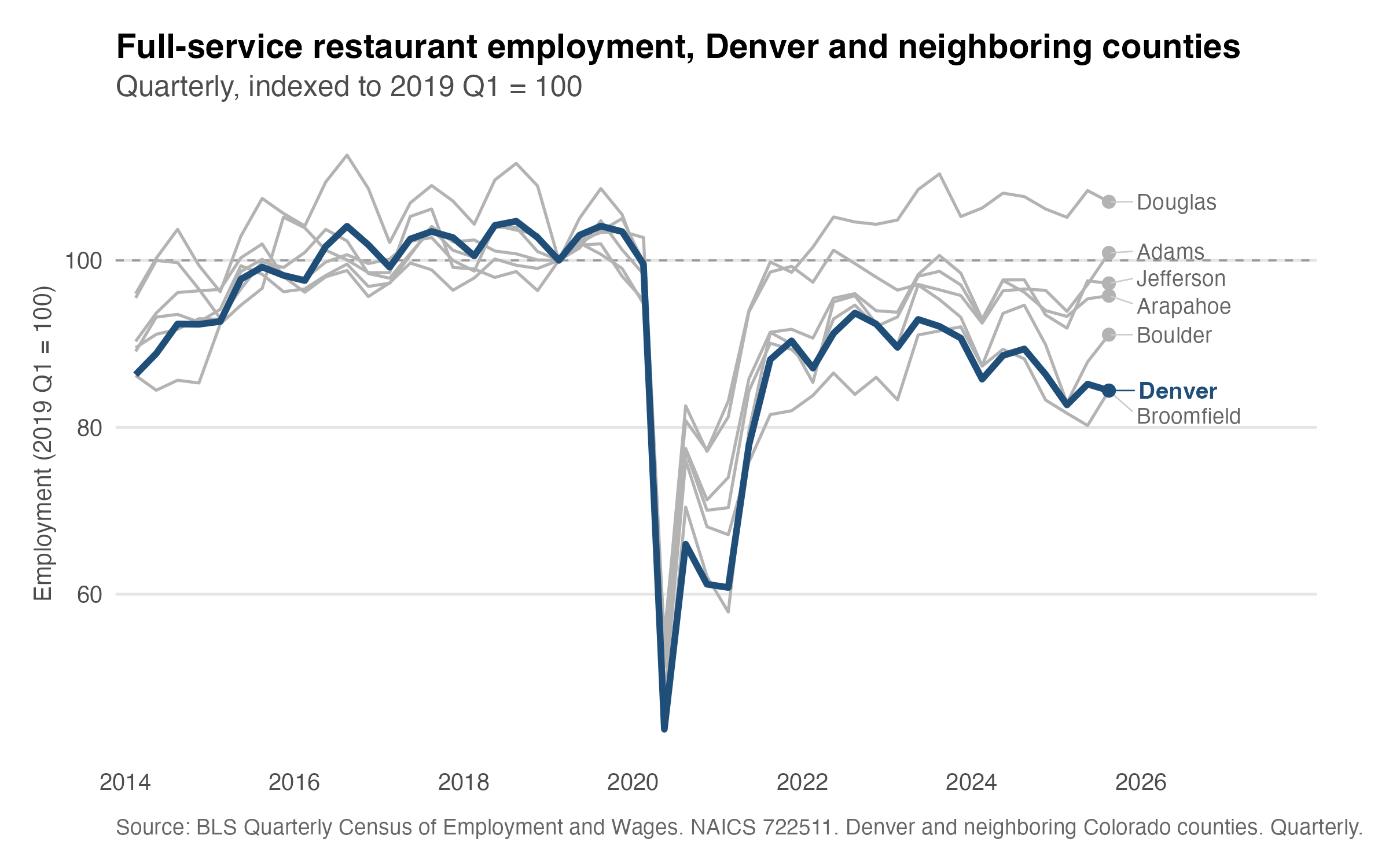
Employment may be down, but maybe restaurants have gotten better at serving the same number of meals with fewer employees. With things like QR code menus, pay with your phone, and limiting what full-service looks like, this is entirely possible. As take-out, delivery, and counter-service options have become more popular, it might also be the case there has been a shift in the composition of the type of restaurants in Denver toward more limited-service which could partially explain declining employment in the full-service sector.

This next chart compares employment in Denver county across two different types of restaurants and restaurant employment in total. Looking first at total restaurant employment, there is still no full recovery to the early 2019 level, but when we look at employment at limited-service restaurants the changes after 2020 look much different. From its low point during the height of the pandemic, limited-service restaurant employment increased back toward its 2019 level and eventually peaked at more than 10% above that 2019 baseline in 2023. Between 2024 and mid-2025, limited-service employment began declining back toward the 2019 level but as of the third quarter of 2025 was still around 5% above the 2019 baseline.

The divergence in employment trends across restaurant types is the first piece of evidence to suggest that not all of Denver’s restaurants are facing the same problem. Things could be better in the limited-service sector but there is no clear slump at least when looking at employment. The slump is more clearly limited to full-service restaurants. With that in mind, we can turn to data on restaurant establishments.

![](/images/posts/whats-going-on-with-denvers-restaurant/img2.png)

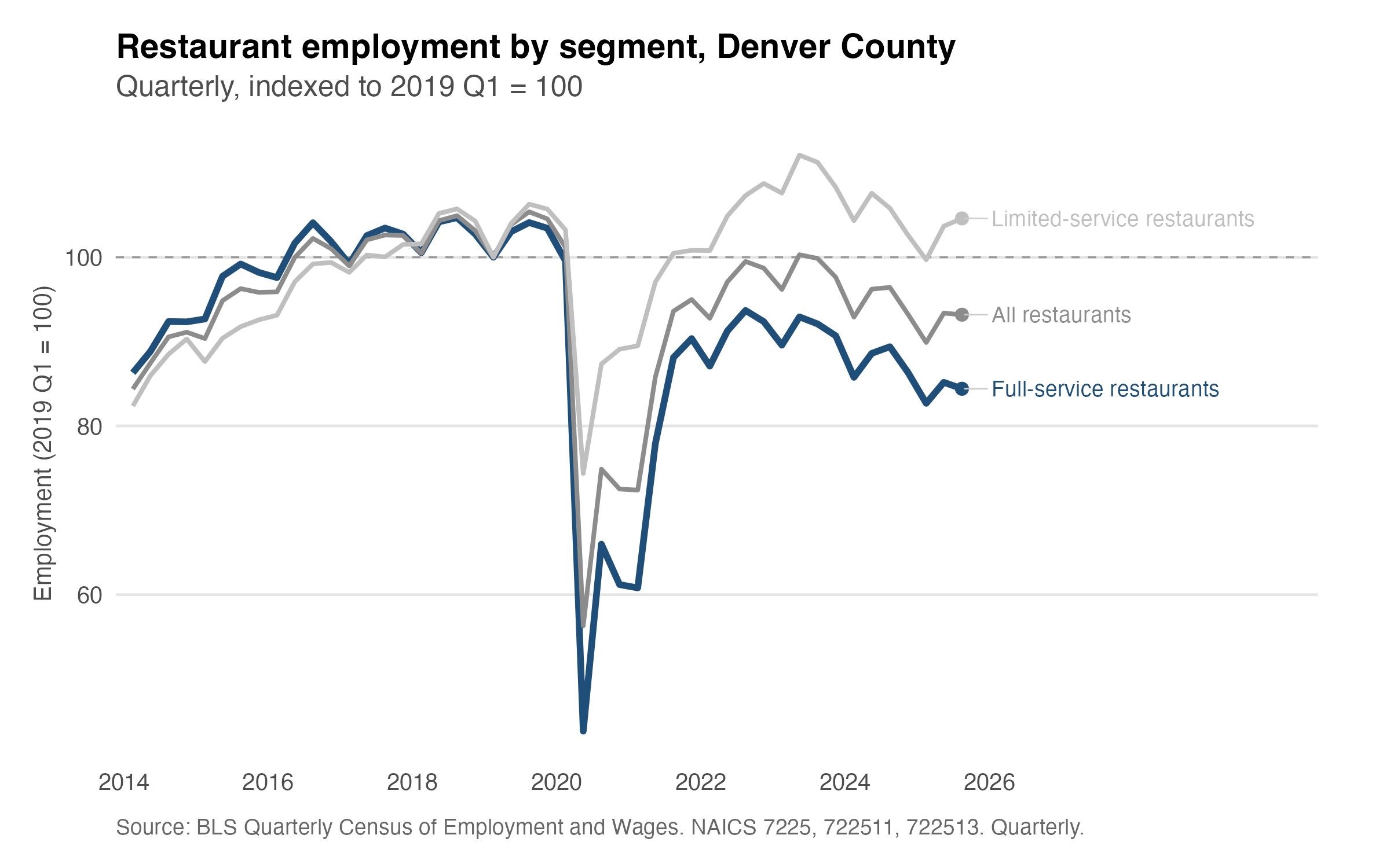
### Number of Restaurants in Denver and Neighboring Counties

The establishments data shows the total number of restaurants in whatever county we are looking at. These numbers count multiple locations of the same restaurant individually. Each Illegal Pete’s counts as 1, for example. One thing to note, however, is that because this is total establishments it is not perfect for determining churn or slump. For that, I would need the number of openings and closings each quarter. What I can say with this data is that if the number of total establishments is declining and falling below the pre-pandemic baseline that is clear evidence of a slump. The main limitation is that if there is limited change in the total number of restaurants this would be consistent with either a high churn environment where openings and closings roughly cancel out or where few new restaurants are opening but there are also not many closures. I cannot determine which is the case looking only at totals.

The establishments data pairs well with employment data in helping determine whether restaurants are figuring out how to stay open with fewer employees or whether there is a decline in both employment and the number of restaurants on net. As done with employment, I will start with a chart showing full-service restaurant establishments in Denver and surrounding counties. Right away the story looks a little different. In Denver, despite initial declines early on in the pandemic, the number of full-service establishments didn’t fall below the 2019 level until 2024. Take out and delivery were still options during the height of the pandemic which meant restaurants could stay open even if with much leaner staff. This suggests that despite employment never recovering, Denver was able to add new restaurants for a few years until the decline we see in 2024.

The steep decline continues through 2025 where the latest data show that the number of full-service establishments sits below the 2019 number. Boulder county also saw a decline in establishments and sits just below the 2019 number of restaurants (a decline of 1 establishment). And Broomfield once again appears to be doing poorly, with the number of restaurants 7% below the 2019 figure. Douglas, Arapahoe, Adams, and Jefferson counties have all seen gains in the number of full-service restaurants since 2019. Those counties appear to have figured out how to deal with declines in restaurant employment while still opening new restaurants, the same can’t be said for Denver and Broomfield. Employment and establishments are down in Denver county. It is safe to say there is a slump for full-service restaurants in Denver. The Broomfield case is interesting and may be worth looking more into, but my focus is going to stay on Denver county.

![](/images/posts/whats-going-on-with-denvers-restaurant/img3.png)

It will be instructive to look at any potential differences in changes in the number of establishments across restaurant types. We observed differential changes in employment across full-service and limited-service restaurants and may see the same thing here. The next chart shows this data for Denver county alone. Again, using 2019 as our 100 value, we can see changes in types of restaurant establishments relative to the first quarter of 2019, pre-pandemic. The change in the number of establishments shows a slight decline during the pandemic across both restaurant types but never below the 2019 baseline. Then, there is an increase in establishments and that is where we begin to see a divergence between full-service and limited-service establishments. At their peak, the number of limited-service restaurants was around 13% higher than in 2019 while full-service restaurants peaked at only around 8% above their 2019 total.

Starting around the same time as the sharp drop in full-service restaurant employment, the number of full-service restaurants begins to decline and this continues through 2025 where the number of restaurants sits around 3% below the 2019 level. The number of limited-service restaurants also declines toward its 2019 level over these quarters but never falls below 100, the most recent data point shows the number of limited-service restaurants is around 3% above the first quarter of 2019. Splitting the restaurant industry into the two sectors shows again that there is not a uniform problem for Denver restaurants. Full-service restaurants are struggling. Employment is dropping and more restaurants are closing than are opening. Limited-service restaurants, on the other hand, are doing better. Employment and establishments are both still above pre-pandemic levels.

![](/images/posts/whats-going-on-with-denvers-restaurant/img4.png)

At this point it seems clear that Denver’s restaurant industry is facing challenges distinct from those in surrounding counties. The exception is Broomfield which is doing about the same as Denver in terms of full-service employment and even worse in terms of the number of full-service restaurants. But we can also move outside Colorado to make comparisons with similar urban counties around the country to see whether these issues are shared with others outside Colorado.

### Restaurant Employment and Numbers in Denver and “Peer” Counties

For another set of comparisons, I chose five additional “peer counties” to compare against Denver on restaurant employment and establishments. These counties (largest cities in parentheses) include Davidson (Nashville, TN), Travis (Austin, TX), Hennepin (Minneapolis, MN), Multnomah (Portland, OR), and Salt Lake (Salt Lake City, UT). Denver is somewhat unusual in this comparison because it’s a consolidated city-county while most others are not, Davidson being the exception. So, these are not perfect comparisons, some counties are much larger than Denver and capture more of the surrounding suburbs but do share some characteristics such as an urban downtown core. The counties also vary in their regulatory and minimum wage environment, some more progressive in policy with higher local minimum wage, others not as much. I am not trying to replicate Denver but choose counties that are more plausible comparisons than say comparing Denver to Los Angeles or New York. These are also counties that are home to cities used in the minimum wage comparison in the *State of Denver’s Restaurants* report across multiple tiers, some with federal minimum wages and others with higher minimum wages. For this section, I will keep it to two charts.

The first chart brings us back to full-service restaurant employment but now comparing Denver county to the peer counties. We already know what has happened in Denver. What is interesting here is that Denver remains among the two worst performers when it comes to employment. The only county to remain well below its 2019 baseline is Portland which is even further below its 2019 baseline. All other comparison counties are within a few percent of their 2019 baseline, suggesting something closer to stability than marked gains or declines. Not great performance, but notably better than Denver and Portland. Denver and Portland are the two poor performance standouts in this set of peer counties. They also share some features of their policy environment, including higher minimum wages, which is one possible explanation among others. Minneapolis also has a high minimum wage but is doing much better than Denver and Portland, minimum wage is only part of the story. I will address this more in Part 2.

![](/images/posts/whats-going-on-with-denvers-restaurant/img5.png)

What about establishments? Basically the same story. Denver is only doing ever so slightly better than Portland but this time all other counties are above their 2019 baseline. So, Denver is not unique in facing challenges across full-service restaurants. Portland is doing worse. But many other counties are not seeing this problem. Some people point to national declines in people eating out or shifting to take-out and delivery, yet we don’t see declines in full-servicce establishments across the board in this comparison set. So there is more to the story than national trends.

![](/images/posts/whats-going-on-with-denvers-restaurant/img6.png)

### Conclusion

So, what is going on with Denver’s restaurants? Two things really. Full-service restaurants are in a genuine slump. Fewer people are being employed and more restaurants are closing. This is a good indication that many restaurant operators cannot hire as many workers as they used to and many are choosing to exit the market. But limited-service restaurants are faring better, they continue to open new restaurants and hire more people. And this looks somewhat distinct to Denver. Many of the surrounding counties are not seeing the same declines in employment or establishments. Even when looking outside Colorado, Denver county is doing worse than other plausible comparisons except Portland which is doing even worse. The remaining questions are why is this happening and what can be done about it on the policy side. This post will be followed up with another looking more at the costs and policy sides of Denver’s restaurant woes.

Part 2 of this post can be [read here](https://reillychandler.substack.com/p/whats-going-on-with-denvers-restaurant-808?r=9i93a).

<a href="#footnote-anchor-1" id="footnote-1" role="doc-backlink" aria-label="Back to reference 1">1</a>

The results for Broomfield are somewhat misleading because the base is so small. The percentage changes are correct but raw magnitudes, especially when compared to Denver are much different. “As bad as Denver” is only as true as performance relative to Broomfield’s own base.